
Table of Contents
Update
I find this blog post gives a better illustration on different optimization algorithms
Stochastic Gradient Descent
SGD is the most basic optimization algorithm for finding the minimum of a function. It simply divides the input data into several minibatch, and then do gradient descent on each of them. Specifically, it computes the gradient for each parameter \( d W \), then updates the parameter using
\[\begin{align} W=W-\alpha d W \end{align}\]Where \( \alpha \) is the learning rate.
Downsides
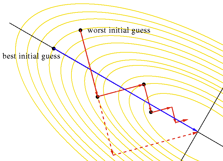
- SGD updates the loss very slowly since the sensitivity of the loss to different weights varies (because the gradient at each point is really a local concept), which results in a zig-zag update(as the top figure shows)
- SGD easily gets stuck at a local minimum or saddle point and these, especially saddle points, are common in high dimensional space
- Gradients coming from minibatch can be noisy, which makes SGD unstable
SGD with Momentum
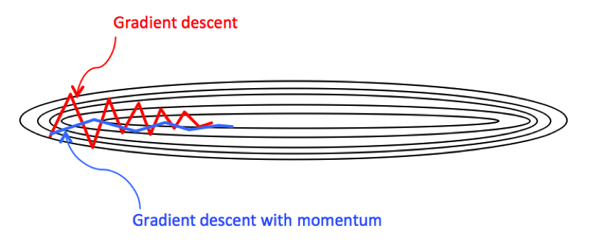
Momentum is a method that helps accelerates SGD in the relevant direction and dampen oscillations, whereby speeding up global convergence. It resorts to the physical concept of velocity to smooth out the gradient descent as follows
\[\begin{align} v &= \beta v+dW\\\ W &=W-\alpha v \end{align}\]The velocity \( v \) defined above is actually the discounted accumulative gradients
\[\begin{align} v_n = dW_n +\beta dW_{n-1} + \beta^2dW_{n-1}\dots \end{align}\]A recommended choice for \( \beta \) is \( 0.9 \)
However, Professor Andrew Ng in this video personally recommends to define the velocity by
\[\begin{align} v = \beta v +(1-\beta)dW \end{align}\]He explains that omitting \( 1-\beta \) indicates the velocity is rescaled when we tune \( \beta \), which in turn leads to further tuning \( \alpha \) if we want the step size to stay in the same scale.
The momentum method dampens oscillations in directions of high curvature by combining gradients with opposite signs. This build up speed in directions with a gentle but consistent gradient.
SGD with Nesterov Momentum
Instead of computing the gradient at the current position \( W \), Nesterov Momentum computes the gradient at \( W’=W+\beta v \). Gross in his lecture justify this method: “it is better to correct a mistake after you have made it.” Mathematically, the velocity and gradient are updated by
\[\begin{align} W'&=W+\beta v\\\ v&=\beta v - \alpha dW'\\\ W&=W+v \end{align}\]I intend to use ‘\( - \)’ when updating \( v \) and ‘\( + \)’ when updating \( W \), which is different from the expression used in the vanilla momentum, since both are commonly seen in literature.
In practice, to align with the original momentum, people would like to use \( W’ \) as the parameter directly instead of \( W \), then the update rule becomes
\[\begin{align} v'&=v\\\ v&= \beta v-\alpha dW'\\\ W'&=W' - \beta v' + (1+\beta)v \end{align}\]Since \( v \) starts with value value \( 0 \), \( W’ \) is initially equal to \( W \). At convergence of optimization, when \( v \) approximates to \( 0 \), \( W’ \) will approximate to \( W \) as well. These observations make \( W’ \) a well-defined replacement for \( W \).
The mathematical reasoning behind these equations is easily told by adding timestamps
\[\begin{align} W'_{t+1}&=W_t+\beta v_{t}\\\ v_{t+1}&=\beta v_t -\alpha dW'_{t+1}\\\ W_{t+1}&=W_t+v_{t+1}\\\ W_{t+1} + \beta v_{t+1} &= W_t +\beta v_t - \beta v_t + \beta v_{t+1} + v_{t+1}\\\ W'_{t+1}&=W'_t-\beta v_t + (1+\beta)v_{t+1} \end{align}\]Adagrad
In a multilayer network, the appropriate learning rates can vary widely between weights; The magnitudes of the gradients are often very different for different layers, especially if the initial wieghts are small. Adagrad, short for adaptive gradient, adjusts the step size so that the parameters that receive high gradients will have their step size reduced, while weights that receive small gradients will have their step size increased. Such a technique helps mitigate the zigzag issue of first-order optimization algorithms. Mathematically, the update rule is
\[\begin{align} \mathcal S&= \mathcal S+dW^2\\\ W&=W-{\alpha \over \sqrt {\mathcal S}+\epsilon}dW \end{align}\]where \( \epsilon \), here for numeric stability, is usually set somewhere in range from \( 10^{-8}\sim 10^{-4} \). The square root operation in the denominator turns out to be very important and without it the algorithm performs much worse
Downside
Adagrad accumulates the squared gradients, which gradually slows down the learning process. It’s desirable in convex problems but usually undesired in deep learning since it’s too aggressive and stops learning too early
RMSprop
RMSprop, short for Root Mean Square propagation, only differs from Adagrad in that it uses a moving average of squared gradients instead. The update rule for RMSprop is
\[\begin{align} \mathcal S&=\rho \mathcal S+(1-\rho)dW^2\\\ m &= \beta m+{\alpha\over\sqrt{\mathcal S+\epsilon}}dW\\\ W&=W-m \end{align}\]where \(\beta\) is momentum, the discounting factor \( \rho \) is typically set to \( 0.9, 0.99, 0.999 \).
Comparing to Adagrad, RMSprop still modulates the step size of each weight based on the magnitudes of its gradients but doesn’t monotonically slow down the learning process
Adam
Adam combines the ideas from both momentum and RMSprop. The update rule is
\[\begin{align} m_1&=\beta_1m_1+(1-\beta_1)dW\\\ m_2&=\beta_2m_2+(1-\beta_2)dW^2\\\ \hat m_1&={m_1/(1-(\beta_1)^t)}\\\ \hat m_2&={m_2/(1-(\beta_2)^t)}\\\ W&=W-{\alpha\over \sqrt {\hat m_2}+\epsilon}\hat m_1 \end{align}\]where \( m_1 \) is equal to the velocity in the momentum and \( m_2 \) is equal to the \( \mathcal S \) in the RMSprop. The recommended values are \( \beta_1=0.9, \beta_2=0.999, \epsilon =10^{-8} \). The third and fourth equations are bias correction — it compensates for the fact that \( m_1 \) and \( m_2 \) are biased at zero in the first few time steps, and thereby leads to large step size at the beginning, which may even not be invertible in some cases. \( t \) is the iteration number.
Adam is currently recommended as the default algorithm to use.
Optimizers in Reinforcement Learning
Most RL papers use either RMSprop or Adam as the optimizer. From this discussion, I summarize several cases that RMSprop may be preferable over Adam:
- The reason RMSprop may be preferable is because of the unclear effect of momentum on RL.
- RMSprop is more stable in non-stationary problems and with RNNs
- RMSprop is more suitable for sparse problems
Based on my recent experience, Adam seems always favored over RMSprop…
\(\epsilon\) in Adaptive Optimizer
\(\epsilon\) is generally chosen from \(10^{-8}\sim10^{-4}\). \(\epsilon\) affects the step size: Large \(\epsilon\) corresponds to small step size, stable training, and slow training progress. For small projects(e.g., mujoco environment), setting \(\epsilon\) to \(10^{-8}\) could speed up the training and get away from local optima. For large projects, \(\epsilon\) is usually set to \(10^{-5}\sim1\) for stable training.
A good timing to tune \(\epsilon \) is after the learning rate is selected. In that case, if you still find the score/accuracy is chattering, increase \(\epsilon\). Generally, \(0.01/\text{batch size}\) is a good start.
References
http://www.cs.toronto.edu/~tijmen/csc321/slides/lecture_slides_lec6.pdf
https://ruder.io/optimizing-gradient-descent/