
Introduction
Reinforcement learning could be hard when the reward signal is sparse. In these scenarios, exploration strategy becomes essentially important: a good exploration strategy not only helps the agent to gain a faster and better understanding of the world but also makes it robust to the change of the environment. In this post, we discuss an exploration method, namely Exploration with Mutual Information(EMI) proposed by Kim et al. in ICML 2019. In a nutshell, EMI learns representations for both observations(states) and actions in the expectation that we can have a linear dynamics model on these representations. EMI then computes the intrinsic reward as the prediction error under the linear dynamics model. The intrinsic reward combined with environment reward forms the final reward function which can then be used by any RL method.
Representation Learning
Representation for states and actions
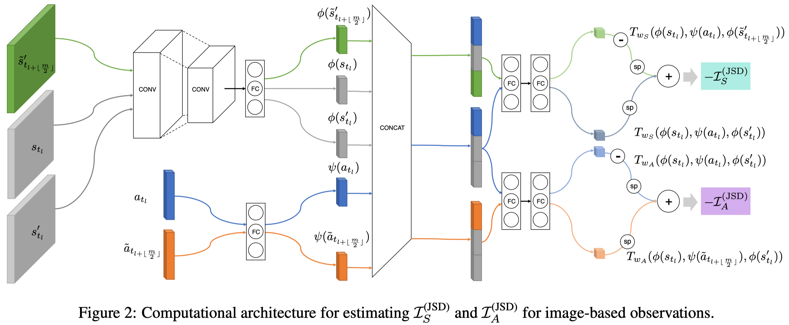
In EMI, we aim to learn representation \(\phi(s):\mathcal S\rightarrow \mathbb R^d\) and \(\psi(a):\mathcal A\rightarrow \mathbb R^d\) for states \(s\) and actions \(a\), respectively, such that the learned representations bear the most useful information about the dynamics. This can be achieved by maximizing two mutual information objectives: 1) the mutual information between \([\phi(s), \psi(a)]\) and \(\phi(s’)\) and 2) the mutual information between \([\phi(s), \phi(s’)]\) and \(\psi(a)\). Mathematically, we maximize the following two objectives
\[\begin{align} \max_{\phi,\psi}\mathcal I([\phi(s),\psi(a)];\phi(s'))&=\mathcal D_{KL}(P^\pi_{SAS'}\Vert P^{\pi}_{SA}\otimes P^\pi_{S'})\tag{1}\\\ \max_{\phi,\psi}\mathcal I([\phi(s),\phi(s')];\psi(a))&=\mathcal D_{KL}(P^\pi_{SAS'}\Vert P^{\pi}_{SS'}\otimes P^\pi_{A})\tag{2} \end{align}\]where \(P^\pi_{SAS’}\) denotes the joint distribution of singleton experience tuples \((s,a,s’)\) starting from \(s_0\sim P_0(s_0)\) and following policy \(\pi\), and \(P^\pi_A\), \(P^\pi_{SA}\), and \(P^\pi_{SS’}\) are marginal distributions. These objectives could be optimized by MINE or DIM we discussed before. In EMI, we follow the objective proposed by DIM, maximizing the mutual information between \(X\) and \(Y\) through Jensen-Shannon divergence(JSD), which is bounded by \(2\log2\):
\[\begin{align} \max \mathcal I(X;Y)&=\max\left(2\log 2+E_{P(x,y)}\left[-\mathrm{sp}(-T(x, y))\right]-E_{p(x)p(y)}\left[\mathrm{sp}(T(x, y))\right]\right)\\\ &= \max\left(2\log 2+E_{P(x,y)}\left[\log\sigma(T(x, y))\right]+E_{p(x)p(y)}\left[\log\sigma(-T(x, y))\right]\right)\\\ where\quad sp(x)&=\log(1+\exp(x))\\\ \sigma(x)&={1\over1+\exp(-x)} \end{align}\]Embedding the linear dynamics model with the error model
Besides the above objectives, EMI also imposes a simple and convenient topology on the embedding space where transitions are linear. Concretely, we also seek to learn the representation of states \(\phi(s)\) and the action \(\psi(a)\) such that the representation of the corresponding next state \(\phi(s’)\) follows linear dynamics, i.e., \(\phi(s’)=\phi(s)+\psi(a)\). Intuitively, this might allow us to offload most of the modeling burden onto the embedding functions.
Regardless of the expressivity of the neural networks, however, there always exists some irreducible error under the linear dynamics model. For example, the state transition which leads the agent from one room to another in Atari environments would be extremely challenging to explain under the linear dynamics model. To this end, the authors introduce the error model \(e(s,a):\mathcal S\times \mathcal A\rightarrow \mathbb R^d\), which is another neural network taking the state and action as input, estimating the irreducible error under the linear model. To train the error model, we minimize the Euclidean norm of the error term so that the error term contributes to sparingly unexplainable occasions. The following objective shows the embedding learning problem under linear dynamics with modeled errors:
\[\begin{align} \min_{e,\phi,\psi}&\Vert e(s,a)\Vert_{2}^2\tag{3}\\\ s.t.\quad \phi(s')&=\phi(s)+\psi(a)+e(s,a) \end{align}\]As a side note, the authors write the above objective in the matrix form, but we stick to the vector form for consistency and simplicity.
The Objective of Representation Learning
Now we put all the objectives together and have
\[\begin{align} \min_{e,\phi,\psi}\underbrace{\Vert \phi(s')-(\phi(s)+\psi(a)+e(s,a))\Vert_2^2}_{\text{linear constraint}}+\lambda_{error}\underbrace{\Vert e(s,a)\Vert_2^2}_{\text{error minimization}}+\lambda_{info}\underbrace{\mathcal L_{info}}_{\text{info loss}}\tag 4 \end{align}\]where \(\mathcal L_{info}\) denotes the negative of the mutual information objectives defined in Eq.\((1)\) and Eq.\((2)\).
In practice, the authors found the optimization process to be more stable when we regularize the distribution of action embedding representation to follow a predefined prior distribution, e.g. a standard normal distribution. This introduces an additional KL penalty \(D_{KL}(P_\psi^\pi\Vert\mathcal N(0,I))\), where \(P_\psi^\pi\) is an empirical normal distribution whose parameters are approximated from a batch of samples. Here we give an exemplar Tensorflow code to demonstrate how this KL divergence is computed from samples.
def compute_sample_mean_variance(samples, name="sample_mean_var"):
    """ Compute mean and covariance matrix from samples """
    sample_size = samples.shape.as_list()[0]
    with tf.name_scope(name):
        samples = tf.reshape(samples, [sample_size, -1])
        mean = tf.reduce_mean(samples, axis=0)
        samples_shifted = samples - mean
        # Following https://en.wikipedia.org/wiki/Estimation_of_covariance_matrices
        covariance = 1 / (sample_size - 1.) * tf.matmul(samples_shifted, samples_shifted, transpose_a=True)

        # Take into account case of zero covariance
        covariance = tf.clip_by_value(covariance, 1e-8, tf.reduce_max(covariance))

        return mean, covariance

def compute_kl_with_standard_gaussian(mean, covariance,
                                      name="kl_with_standard_gaussian"):
    """ Compute KL(N(mean, covariance) || N(0, I)) following
https://en.wikipedia.org/wiki/Multivariate_normal_distribution#Kullback%E2%80%93Leibler_divergence
    """
    vec_dim = mean.shape[-1]
    with tf.name_scope(name):
        trace = tf.trace(covariance)
        squared_term = tf.reduce_sum(tf.square(mean))
        logdet = tf.linalg.logdet(covariance)
        result = 0.5 * (trace + squared_term - vec_dim - logdet)

    return result
The authors also tried to regularize the state embedding, but they found it renders the optimization process much more unstable. This may be caused by the fact that the distribution of states is much more likely to be skewed than the distribution of actions, especially during the initial stage of optimization.
Intrinsic Reward
We now define intrinsic reward as the prediction error in the embedding space:
\[\begin{align} r_i(s_t,a_t,s'_t)=\Vert \phi(s_t)+\psi(a_t)+e(s_t,a_t)-\phi(s_{t+1})\Vert^2_2 \end{align}\]This formulation incorporates the error term and makes sure we differentiate the irreducible error that does not contribute as the novelty. We combine it with extrinsic reward to get our final reward function used to train an RL agent
\[\begin{align} r(s,a,s'_t)=r_e(s,a,s'_t)+\eta r_i(s_t,a_t,s'_t) \end{align}\]where \(\eta\) is the intrinsic reward coefficient.
Algorithm
Now that we have defined the objective for representation learning and the reward function for reinforcement learning, it is straightforward to see the algorithm
\[\begin{align} &\mathbf {Algorithm\ EMI}\\\ &\mathbf {while}\ not\ done:\\\ &\quad \mathrm{Collect\ samples\ }\{(s_t,a_t,r^e_t,s_{t+1})\}_{t=1}^n\ \mathrm{with\ policy\ \pi_\theta}\\\ &\quad \mathrm{Compute\ intrinsic\ rewards\ }\{r^i(s_t,a_t,s_{t+1})\}_{t=1}^n\\\ &\quad \mathbf{For\ } j=1,...M:\quad\\\ &\quad\quad \mathrm{Sample\ a\ minibatch\ }\{(s_t, a_t, s_{t+1})\}_{t=1}^m\ \mathrm{from\ replay\ buffer}\\\ &\quad\quad \mathrm{Update\ representation\ model\ \phi, \psi\ and\ error\ model}\ e\mathrm{\ by\ minimizing\ Eq.(4)}\\\ &\quad \mathrm{Augment\ the\ intrinsic\ rewards\ with\ environment\ reward\ }r=r^e+r^i\\\ &\quad \mathrm{Update\ the\ policy\ network\ using\ any\ RL\ method} \end{align}\]Experimental Results
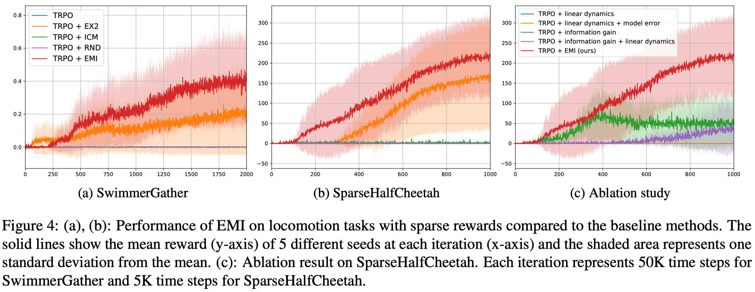
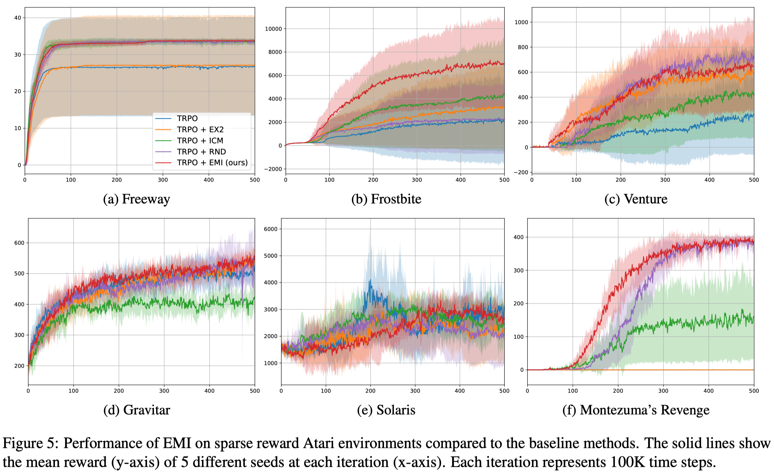
We can see that EMI indeed achieves better results in challenging low-dimensional locomotion tasks despite its high variance. However, it kind of ties with many previous methods in vision-based tasks. All in all, EMI is a wildly applicable method that achieves satisfactory performance.
References
-
Hyoungseok Kim, Jaekyeom Kim, Yeonwoo Jeong, Sergey Levine, Hyun Oh Song. EMI: Exploration with Mutual Information
-
code: https://github.com/snu-mllab/EMI