
Introduction
On-policy algorithms such as PPO has been successfully applied to solve many practical tasks. Lying beneath the success are numerous decision choices that greatly affect the performance but are understated in the corresponding literature. In this post, we follow the footprint of Andrychowicz et al. 2020 to discuss several design decisions on on-policy reinforcement learning.
TL; DR
- Try PPO loss first with \(\epsilon=.25\) for multi-pass on-policy training.
- For feature-based continuous control tasks, \(\tanh\) performs better than \(\text{ReLU}\)
- Initialize the policy head with small weights(\(100\times\) smaller than others) and the standard deviation to a small value
- Apply observation normalization and gradient clipping
- Use large experience chunk and large mini-batch
- Do not gather too much transitions at each iteration unless you increases the mini-batch size
- Recompute advantage and shuffle data for each epoch
- Use Adam with \(lr=3e-4\) for a start
Environments
Experiments are done on 5 continuous control environments from OpenAI’s gym: Hopper, HalfCheetah, Walker2d, Ant, Humanoid.
Policy Losses
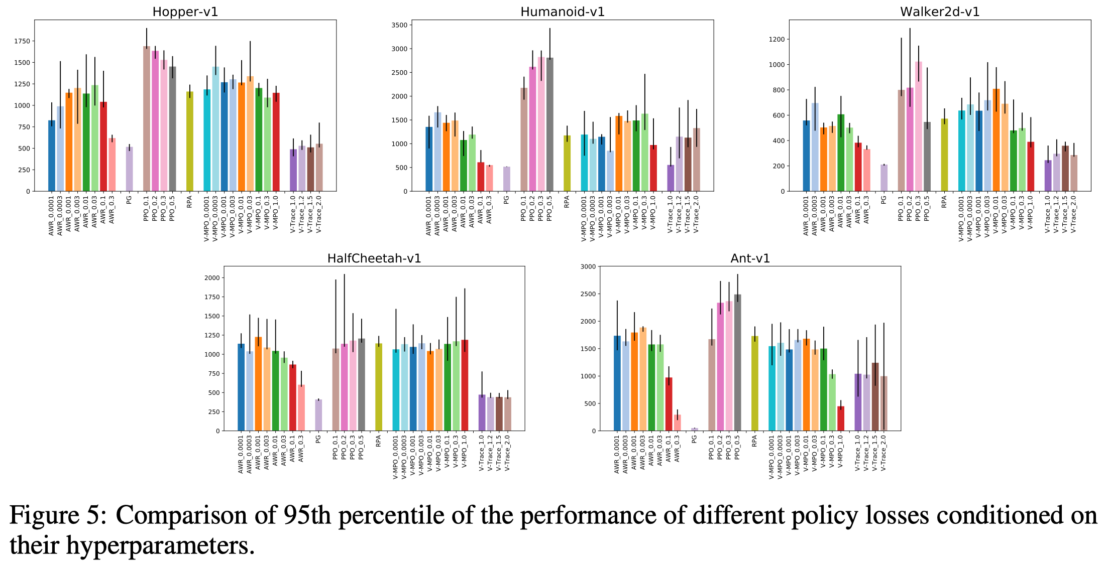
Andrychowicz et al. 2020 investigate six losses: vanilla policy gradient (PG), V-trace, PPO, AWR, V-MPO, and RPA(see the appendix for a brief discussion on these losses); experiments show that PPO is less sensitive to choices of other hyperparameters and consistently outperforms other losses. However, this does not mean that we should use PPO blindly as some losses are designed for different purposes. For example, V-trace is targeted at near-on-policy data in a distributed setting and AWR at off-policy data.
For PPO, they also observe that \(\epsilon=0.2\) and \(\epsilon=0.3\) performs reasonably well in all environments but that lower (\(\epsilon=0.1\)) or higher (\(\epsilon=0.5\)) values give better performance on some of the environments.
Recommandation: Use the PPO loss. Start with the clipping threshold set to \(0.25\) but also try lower and higher values if possible.
Thoughts. It’s quite surprising that V-trace performs so worse in their experiments. This is likely caused by the inability of V-trace to handle off-policy data, due to multiple passes over experience. Note that V-trace trade off variance of importance sampling for a biased estimate, converging to a policy that interpolates the optimal and behavior policies.
Network Architecture
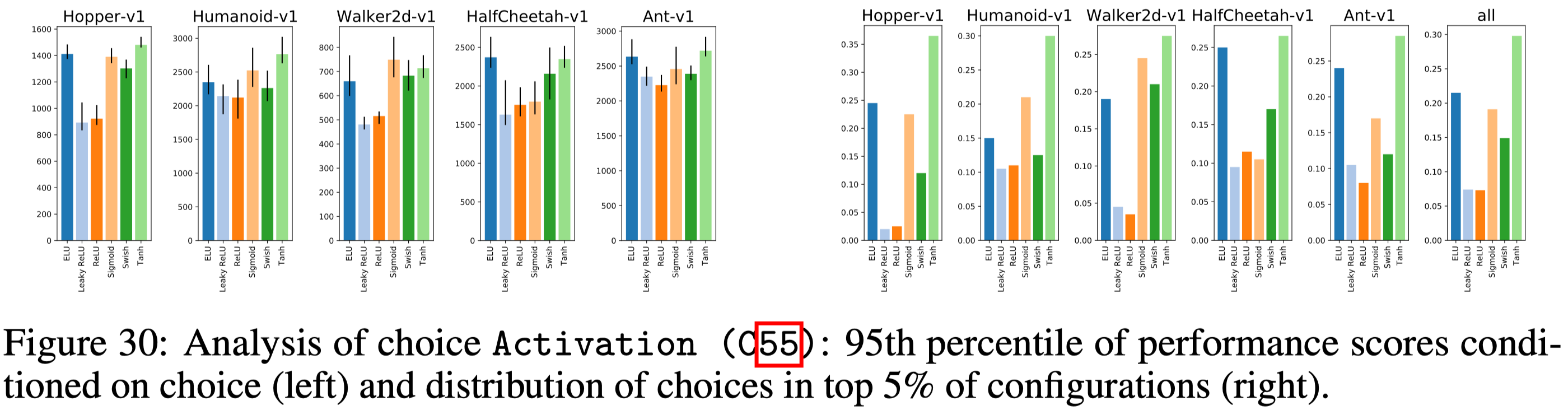
Networks too large or too small could significantly impair the performance. Surprisingly, they find \(\tanh\) performs best and \(\text{ReLU}\) performs worst (Figure 30). This is contrast to my experience on image-based tasks, where I find \(\text{ReLU}\) outperforms other activations.
Policy initialization matters: initializing the action distribution with mean \(0\) and standard deviation \(0.5\) regardless of input appears most fruitful on the considered environments. This can be achieved by initializing the policy MLP with smaller weights in the last layer.
They find that network initialization does not matter much (except that He initialization appears to be suboptimal). This is again contrast to what I observe in image-based tasks, where I find Glorot initialization significantly outperforms others such as He and orthogonal initialization.
No benefit is found to learn state-dependent standard deviation. No difference is spotted using exponentiation or softplus when transforming the standard deviation to ensure non-negativity.
Recommendation: Initialize the last policy layer with \(100\times\) smaller weights. Use softplus to transform network output into action standard deviation and add a (negative) offset to its input to decrease the initial standard deviation of actions. Tune this offset if possible.
Normalization and Clipping
Observation normalization is crucial for good performance but the clipping after normalization seems less important.
Value normalization normalizes the value function targets and denormalizes the value function accordingly to obtain predicted value: \(\hat V=v_\mu+V\max(v_\sigma, 10^{-6})\), where \(v_\mu\) and \(v_\sigma\) are empirical mean and standard deviation, respectively. Value function normalization influences the performance very strongly, but its environment-dependent; it is crucial for good performance on HalfCheetah and Humanoid, helps slightly on Hopper and Ant and significantly hurts the performance on Walker2d.
Per-batch advantage normalization, which usually done in PPO, seems not affect the performance. I suspect that advantage normalization helps when the raw advantage leads to large or negligible policy changes. Therefore, it’s better to monitor the (approximate) KL divergence between the current policy and behavior policy at the end of each training epoch.
Gradient clipping might slightly help.
Advantage Estimation
GAE and V-trace appears to perform better than N-step returns, which indicates that it is beneficial to combine the value estimators from multiple time steps. However, no significant performance difference between GAE and V-trace is spotted.
Huber loss performs worse than MSE loss in all environments. These show outliners in value function generally help. Surprisingly, value clipping implemented in OpenAI baselines’ PPO generally hurts the performance—in their experiments, it only helps in some cases when \(\epsilon=1\). However, my experiences with PPO in Procgen indicates value clipping is sometimes helpful. I conjecture the difference is introduced because 1) Andrychowicz et al. 2020 do not apply reward normalization in their experiments—when the reward scale is large, \(\text{clip}(v - v_{old}, -\epsilon, \epsilon)\) could be too conservative as \(\epsilon\) is usually small; 2) outliners in value loss may compromise the representation learned by the shared CNN.
Training Setup
As the number of environments increases, performance decreases sharply on some environments. This is likely caused by shortened experience chunks(to maintain the same amount of transition gathered in each iteration) and early value bootstrapping, consistent with the observation in advantage estimation.
Increasing the minibatch size does not appear to hurt the performance, which suggests that we can speed up iteration by increasing the minibatch size.
It is helpful to recompute the advantage and shuffle transitions for every pass over the data instead of doing them once per iteration.
The number of transitions gathered in each iteration influences the performance significantly and we should tune this for each environment.
Optimizers
Use Adam with \(3e-4\) and \(\beta_1=0.9\) as a start and tune the learning rate if possible.
Regularization
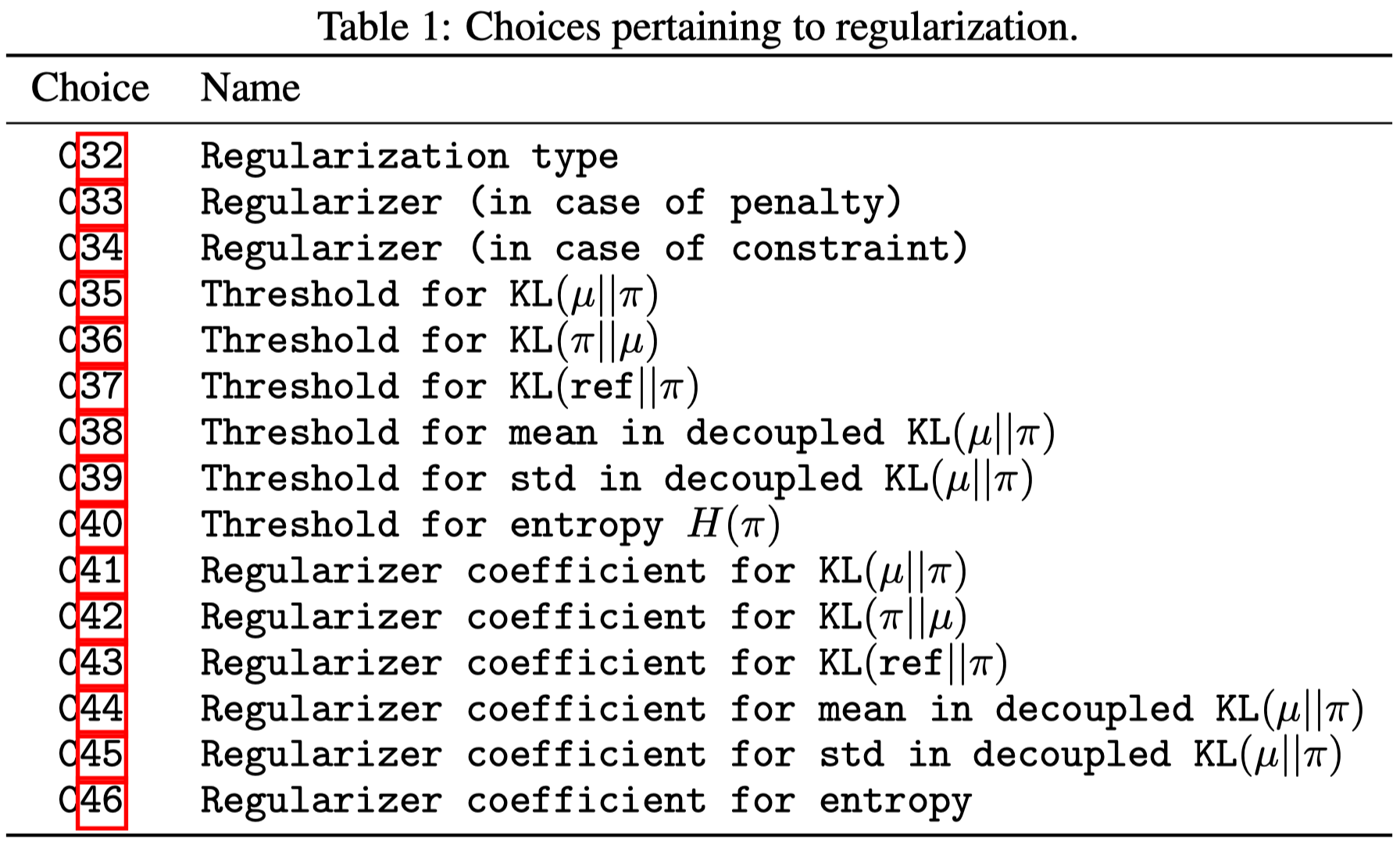
A variety policy regularization techniques(Table 1) are experimented, but none of them is found particularly useful across all environments. This may be due to the simplicity of the environments, for which the PPO loss is sufficient to enforce the trust region and careful policy initialization is enough to guarantee good exploration.
References
Andrychowicz, Marcin, Anton Raichuk, Piotr Stańczyk, Manu Orsini, Sertan Girgin, Raphael Marinier, Léonard Hussenot, et al. 2020. “What Matters In On-Policy Reinforcement Learning? A Large-Scale Empirical Study,” no. 1. http://arxiv.org/abs/2006.05990.
Supplementary Materials
Policy losses
Let \(\pi\) denote the policy being optimized, and \(\mu\) the behavioral policy. Moreover, let \(\hat A_t^\pi\) and \(\hat A_t^\mu\) be some estimators of the advantage at timestep \(t\) for the policies \(\pi\) and \(\mu\). Any newly introduced symbol below are hyperparameters.
Policy gradients: \(\mathcal L_{PG}=-\log\pi(a_t\vert s_t)\hat A_t^\pi\)
V-trace: \(\mathcal L_{V-trace}=\text{sg}(\rho_t)\mathcal L_{PG}\), where \(\rho_t=\min({\pi(a_t\vert s_t)\over\mu(a_t\vert s_t)},\bar\rho)\) is an importance weight truncated at \(\bar\rho\), \(\text{sg}(\cdot)\) is the stop_gradient operator.
Proximal Policy Gradient (PPO): \(\mathcal L_{PPO}=-\min\bigl({\pi(a_t\vert s_t)\over\mu(a_t\vert s_t)}\hat A_t^\pi, \mathrm{clip}({\pi(a_t\vert s_t)\over\mu(a_t\vert s_t)}, {1\over1+\epsilon}, 1+\epsilon)\hat A_t^\pi\bigr)\), where we use \(1\over 1+\epsilon\) instead of \(1-\epsilon\) as the lower bound because the former is more symmetric.
Advantage-Weighted Regression (AWR): \(\mathcal L_{AWR}=-\log\pi(a_t\vert s_t)\min(\exp(A_t^\mu/\beta),\omega)\). It can be shown that for \(\omega=\infty\) it corresponds to an approximate optimization of the policy \(\pi\) under a constraint of the form \(D_{KL}(\pi\Vert \mu)<\epsilon\) where the KL bound \(\epsilon\) depends on the exponentiation temperature \(\beta\). Notice that different from previous methods, AWR computes the advantage estimator from the behavior policy. AWR was proposed mostly as an off-policy RL algorithm.
On-Policy Maximum a Posteriori Policy Optimization (V-MPO): This policy loss is the same as AWR with the following differences: (1) exponentiation is replaced with the softmax operator and there is no clipping with \(\omega\) ; (2) only samples with the top half advantages in each batch are used; (3) the temperature \(\beta\) is treated as a Lagrange multiplier and adjusted automatically to keep a constraint on how much the weights (i.e. softmax outputs) diverge from a uniform distribution with the constraint threshold \(\epsilon\) being a hyperparameter. (4) A soft constraint on \(D_{KL}(\mu\Vert \pi)\) is added. In our experiments, we did not treat this constraint as a part of the V-MPO policy loss as policy regularization is considered separately.
Repeat Positive Advantages (RPA): \(\mathcal L_{RPA}=-\log\pi(a_t\vert s_t)[A_t>0]\).