
Introduction
We discuss P3O, an policy gradient method that utilizes both on-policy and off-policy data.
TL; DR
-
P3O utilizes the effective sample size(ESS) to determine how to handle a minibatch of off-policy data.
-
P3O uses the following objective which exploits both on- and off-policy data.
where \(c=ESS\) and \(\lambda=1-ESS\)
Effective Sample Size
Given a dataset \(X={x_1,x_2,\dots,x_N}\), and two densities \(p(x)\) and \(q(x)\) with \(p(x)\) being absolutely continuous with respect to \(q(x)\), the effective sample size is defined as the number of samples from \(p(x)\) that would provide an estimator with a performance equal to that of the importance sampling estimator \(w(x)=p(x)/q(x)\) with \(N\) samples. Because we apply importance sampling when computing policy gradient from off-policy data, we use the following normalized Kish’s effective sample size
\[\begin{align} ESS={1\over N}{\Vert w(X)\Vert_1^2\over \Vert w(X)\Vert_2^2}={1\over N}{\left(\sum_xw(x)\right)^2\over(\sum_xw(x)^2)} \end{align}\]where \(1\over N\) normalize the effective sample size so that \(ESS\in[0, 1]\).
In P3O, ESS is used as an indicator of the efficacy of updates to \(\pi\) with samples drawn from the behavior policy \(\mu\). If the ESS is large, \(\pi\) is similar to \(\mu\), and we can confidently use data from \(\mu\) to update \(\pi\). Otherwise, we truncate the importance ratio to prevent large negative effect from updates incurred by off-policy data from \(\mu\).
P3O
P3O augments the traditional policy gradient objective with off-policy objectives, which results in
\[\begin{align} \mathcal J(\pi)=\mathbb E_{_\pi}[A(s,a)+\alpha\mathcal H(\pi)]+\mathbb E_{\mu}[\min(\rho,c)A(s,a)]-\mathbb \lambda E_\mu[ D_{KL}(\mu\Vert \pi)] \end{align}\]where \(\rho={\pi\over\mu}\) is the importance ratio, \(c\) is the truncation threshold we’ll discuss later. The corresponding gradient is
\[\begin{align} \mathbb E_{\pi}[A(s,a)\nabla\log\pi+\alpha\nabla \mathcal H(\pi)]+\mathbb E_{\mu}[\min(\rho,c)A(s,a)\nabla\log\pi-\lambda\nabla D_{KL}(\mu\Vert\pi)] \end{align}\]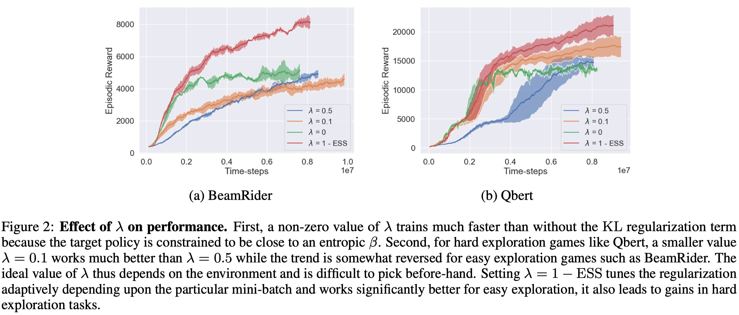
Adaptive KL Coefficient and Truncation Threshold
The novelty of P3O lies in the choice of threshold \(c\) and KL regularization coefficient \(\lambda\).
Adaptive \(\lambda\). When \(\pi\) is far from \(\mu\), we would like \(\lambda\) be large so as to push them closer. If they are too similar to each other, it entails that we could be more aggressive with a smaller \(\lambda\). As the normalized effective sample size provides a good measure of the distance between \(\pi\) and \(\mu\), we set
\[\begin{align} \lambda=1-ESS \end{align}\]Figure 2 shows the effect of \(\lambda\) on performance. Note that \(\lambda\) also influences the entropy of \(\pi\)—A large \(\lambda\) leads to \(\pi\) with higher entropy as it pushes \(\pi\) to be close to the previous policy, which is high entropic because of its mixing nature.
Adaptive \(c\). The truncation threshold \(c\) controls the bias-variance trade-off. The larger \(c\) is the less bias and the higher variance the policy gradient is of. A small \(c\) effectively reduces the variance introduced by the importance ratio but incurs some bias. We would like \(c\) be small when \(\pi\) is far from \(\mu\) to reduce the potentially high variance incurred by the importance ratio. Therefore, it is “intuitive” to set
\[\begin{align} c=ESS \end{align}\]However, Fakoor et al. 2019 do not perform any experiments to verify the efficacy of \(c=ESS\).
Discussion on The KL Penalty
We first show that the KL penalty in P3O slows down optimization. For an optimization problem \(x^*=\arg\min_xf(x)\), the gradient update \(x_{k+1}=x_{k}-\alpha\nabla f(x_k)\) can be written as
\[\begin{align} x_{k+1}=\arg\min_y\left<\nabla f(x),y\right>+{1\over2\alpha}\Vert y-x_k\Vert^2 \end{align}\]One can prove it by setting the gradient to zero. A penalty with respect to all previous iterates \({x_1,x_2\dots,x_k}\) can be written as
\[\begin{align} x_{k+1}=\arg\min_y\left<\nabla f(x),y\right>+{1\over2\alpha}\sum_{i=1}^k\Vert y-x_k\Vert^2 \end{align}\]Setting the gradient to zero, we obtain the update equation
\[\begin{align} x_{k+1}={1\over k}\sum_{i=1}^kx_i-{\alpha\over k}\nabla f(x_k) \end{align}\]which has a vanishing step-size as \(k\rightarrow\infty\). We would expect such a vanishing step-size of the policy gradient to hurt performance. On the other hand, as the behavior policy \(\mu\) is a mixture of previous policies, which is highly entropic, penalizing \(\pi\) against \(\mu\) encourages \(\pi\) to explore.
\(\lambda=1-ESS\) provides a way to adaptively tune the coefficient of the KL penalty based on the extent to which the data is off the policy.
Algorithm
\[\begin{align} &\text{Rollout }K\text{ trajectories }\tau\text{ for }T\text{ time-steps each}\\\ &\text{Compute return and advantages using GAE}\\\ &\mathcal D\leftarrow \mathcal D\cup\tau\\\ &\text{Perform on-policy update with }\tau\\\ &\xi\leftarrow \text{Poisson}(m)\\\ &\textbf{for } i\le \xi\textbf{ do}\\\ &\quad\text{Perform off-policy update with }\{\tau_1,\dots,\tau_n\}\sim\mathcal D\\\ \end{align}\]For Atari games, \(K=16\), \(T=16\), \(m=2\), and \(n=6\).
References
Fakoor, Rasool, Pratik Chaudhari, and Alexander J. Smola. 2019. “P3O: Policy-on Policy-off Policy Optimization.” ArXiv.