
Introduction
In conventional reinforcement learning, our aim is generally to take the optimal actions so as to maximize the expected total rewards. This may not always be desirable and is especially fragile to changes in the environment because of the deterministic nature of the learned policy. In this post, we will consider a probabilistic graphical model (PGM) that enables us to reason the stochastic behavior and do inference. Although we do not present any practical algorithms in this post, the probabilistic view of control presented in this post is important and we will see in many of our future posts that many modern algorithms heavily exploit this idea.
A Probabilistic View of Control Problems
Model Definition
We could consider control problems as the following temporal probabilistic graphical model (PGM)
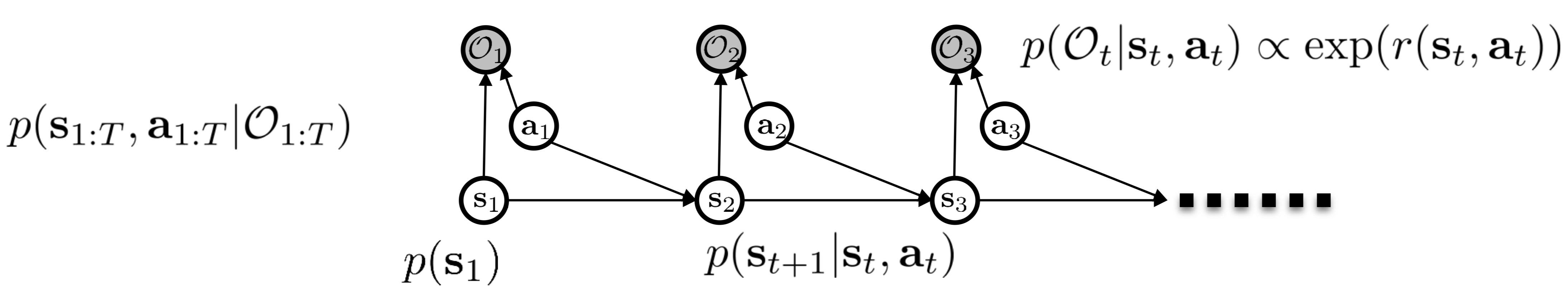
where \(s_1, s_2, \dots\) and \(a_1, a_2, \dots\) are hidden variables, representing states and actions, respectively; \(O_1, O_2,\dots\) are observed binary variables, which indicate whether the corresponding state and action are optimal.
As with the regular Hidden Markov Model(HMM), we further assume that the transition probabilities \(p(s_{t+1}\vert s_t,a_t)\) are known. The emission probabilities that a given state and action pair is optimal, \(p(O_t\vert s_t,a_t)\), is proportional to \(\exp(r(s_t,a_t))\), where \(r(s_t,a_t)\) is the reward function (later we’ll see this choice actually helps align this PGM with concepts discussed in reinforcement learning). Our probabilistic inference problem is to figure out the trajectory distribution given the optimality sequence \(O_{1:T}\), i.e., \(p(\tau\vert O_{1:T})\). In the following discussion, we assume \(O_{1:T}\) are all \(1\) so that \(p(\tau\vert O_{1:T})\) indicates the probability of a trajectory given that it is optimal. In that sense, we now are actually trying to answer the question that what the trajectory might be if the agent acts optimally.
To get a better sense of what the objective is related to, we apply the Bayes’ rule:
\[\begin{align} p(\tau|O_{1:T})&\propto p(\tau)p(O_{1:T}|\tau)\\\ &\propto p(\tau)\prod_t \exp(r(s_t,a_t))\\\ &=p(\tau)\exp\left(\sum_tr(s_t,a_t)\right)\tag {1} \end{align}\]where \(p(\tau)\) is the probability of the trajectory without any assumption of optimality. The exponential term brings a nice interpretation to \(p(\tau\vert O_{1:T})\) that given an optimality sequence, the probability that a trajectory is happening is proportional to the exponential of the total rewards, or in other words, the likelihood of a suboptimal trajectory decays exponentially as the total rewards decrease.
Benefits of Probabilistic Model
Before diving into details of the probabilistic inference, let us see why this probabilistic model would be of interest
- It allows us to model suboptimal behavior, which is important for inverse reinforcement learning
- It, as we will see soon, allows us to apply probabilistic inference algorithms to solve control and planning problems
- It provides an explanation for why stochastic behavior might be preferred: stochastic behavior provides some extra exploration whereby the agent is more robust to mistakes or changes of environment, which make it more suitable for transfer learning.
Probabilistic Inference
In this section, we will learn backward and forward messages and see how they help to do inference.
Backward Messages
Define the backward messages as the probability of optimality from the current timestep until the end conditioned on the current state and action, \(\beta (s_t,a_t)=p(O_{t:T}\vert s_t,a_t)\). It can be computed as
\[\begin{align} \beta(s_t,a_t)&=p(O_{t:T}|s_t,a_t)\\\ &=\int p(O_{t:T}|s_t,a_t,s_{t+1})p(s_{t+1}|s_t,a_t) d{s_{t+1}}\\\ &=\int p(O_t|s_t,a_t)p(O_{t+1:T}|s_{t+1})p(s_{t+1}|s_t,a_t)ds_{t+1}\\\ &=p(O_t|s_t,a_t)\mathbb E_{s_{t+1}\sim p(s_{t+1}|s_t,a_t})[p(O_{t+1}|s_{t+1})]\tag {2} \end{align}\]where the transition and emission probabilities are known. We represent the unknown term as \(\beta(s_{t+1})\), which can be computed as
\[\begin{align} \beta(s_{t+1})&=p(O_{t+1:T}|s_{t+1})\\\ &=\int p(O_{t+1:T}|s_{t+1},a_{t+1})p(a_{t+1}|s_{t+1})da_{t+1}\\\ &=\mathbb E_{a_{t+1}\sim p(a_{t+1}|s_{t+1})}[\beta(s_{t+1},a_{t+1})]\tag {3} \end{align}\]where \(p(a_{t+1}\vert s_{t+1})\) is the action prior, which does not depend on the the optimality sequence. This shows a probabilistic way of computing \(\beta\), and now we can formulate the backward message algorithm as follows
\[\begin{align} &\mathbf {Backward\ Message\ Algorithm}\\\ &\quad\beta(s_{T+1})=1\\\ &\quad\mathrm {for\ } t=T\mathrm{\ to\ }1:\\\ &\quad\quad \beta(s_t,a_t)=p(O_t|s_t,a_t)\mathbb E_{s_{t+1}\sim p(s_{t+1}|s_t,a_t)}[\beta(s_{t+1})]\\\ &\quad\quad \beta(s_t)=\mathbb E_{a_{t+1}\sim p(a_{t}|s_{t})}[\beta(s_{t},a_{t})] \end{align}\]We can actually align these backward messages with the value functions used in reinforcement learning. Recall that the emission probability is defined to be proportional to the exponential of the reward function, \(p(O_t\vert s_t,a_t)\propto\exp(r(s_t,a_t))\). This hints that value functions are of logarithmic scale of the backward messages. Let \(V(s_t)=\log \beta(s_t)\) and \(Q(s_t, a_t)=\log\beta(s_t,a_t)\) and assume the action prior \(p(a_t\vert s_t)\) to be uniform, which, we’ll see later, does not change our discussion here. Then we have \(V(s_t)\) as
\[\begin{align} V(s_t)=\log\int\exp\big(Q(s_t,a_t)\big)da_t\tag {4} \end{align}\]Here we kind of abuse the equal sign, but it is fine since the uniform prior action distribution is a constant to all action. A nice property of Equation \((4)\) is that as \(Q(s_t, a_t)\) gets larger, \(V(s_t)\) gets closer to \(\max_{a_t}Q(s_t,a_t)\) thanks to the exponential inside the integral. Because of this nice property, we sometimes call ‘\(\log\int\exp\)’ the ‘soft max’ operator in contrast to the hard max.
Next, let us consider \(Q(s_t, a_t)\)
\[\begin{align}Q(s_t,a_t)&=r(s_t,a_t)+\log \mathbb E_{s_{t+1}\sim p(s_{t+1}|s_t,a_t)}[\exp(V(s_{t+1}))]\tag {5}\\\ &\ge r(s_t,a_t)+\mathbb E_{s_{t+1}\sim p(s_{t+1}|s_t,a_t)}[V(s_{t+1})] \end{align}\]where the inequality takes because of Jensen’s inequality. The right hand side of the inequality is the standard definition of the \(Q\)-function defined by the Bellman backup, which is smaller than \(Q(s_t,a_t)\) defined here. Intuitively, we could consider it as if the transition happening here is optimistic in that it weighs more on large \(V(s_{t+1})\) than the true dynamics does. In deed, the underlying transition is more like \(p(s_{t+1}\vert s_t, a_t, O_{1:T})\). Such optimism creates risk seeking behavior; if an agent behaves according to this \(Q\)-function, it might take actions that have a little chance to gain a high reward but on average receive low rewards.
With the definition of \(V(s_t)\) and \(Q(s_t, a_t)\), we can transfer the backward message algorithm to a “soft” version of value iteration algorithm
\[\begin{align} &\mathbf{Soft\ Value\ Iteration\ algorithm}\\\ &\quad V(s_{T+1})=0\\\ &\quad \mathrm{for\ }t=T\mathrm{\ to\ } 1:\\\ &\quad\quad Q(s_t,a_t)=r(s_t,a_t)+\log \mathbb E_{s_{t+1}\sim p(s_{t+1}|s_t,a_t)}[\exp(V(s_{t+1}))]\\\ &\quad\quad V(s_t)=\log \int \exp\big(Q(s_t,a_t)\big)da_t \end{align}\]This soft value iteration algorithm will be problematic in the control setting, because it somewhat changes the underlying dynamics when updating the \(Q\)-function. But it is okay for our inference task, and we will see in the next post that we can make it work in control by simply replacing the \(Q\)-function update with the standard Bellman backup.
When Prior Action is Not Uniform
In the previous discussion, we intentionally take the action prior as a uniform distribution so that we can ignore it as a constant, but it does not need to be the case. If we put the action prior back into Eq.\((4)\), we would have
\[\begin{align} V(s_t)=\log \int\exp\big(Q(s_t,a_t)+\log p(a_t|s_t)\big)da_t \end{align}\]Let \(\tilde Q(s_t,a_t)=r(s_t,a_t)+\log p(a_t\vert s_t)+\log \mathbb E_{s_{t+1}\sim p(s_{t+1}\vert s_t,a_t)}[\exp(V(s_{t+1}))]\), then we have
\[\begin{align} V(s_t)=\log\int\exp(\tilde Q(s_t,a_t))da_t \end{align}\]This suggests that we can always fold the action prior into the reward function and the uniform action prior can be assumed without loss of generality([1], [2]). Notice that folding the action prior into the reward function should be done at the environment design stage but not the learning stage as the later introduces a fundamentally different task objective. Consider a task where the agent only receives a positive reward when reaching a goal and otherwise no reward is given. If we add the logarithm of the action priors during the learning, this will introduce negative rewards to all intermediate states since the logarithm of the action priors are negative. As a result, the agent will learn to terminate an episode early on without ever finding the reward. In fact, we usually do not incorporate the prior into the reward function but instead directly regularize our policy against it, which is known as the KL-regularized RL.
Probabilistic Policy
The policy distribution given the optimality can simply be computed from the backward messages:
\[\begin{align} \pi(a_t|s_t)=p(a_t|s_t,O_{t:T})&={p(a_t,s_t, O_{t:T})\over p(s_t,O_{t:T})}\\\ &={p(O_{t:T}|s_t,a_t)p(a_t|s_t)\over p(O_{t:T}|s_t)}\\\ &\propto{\beta(s_t,a_t)\over \beta(s_t)}\tag {6} \end{align}\]where the action prior is assumed uniform as before and is ignored as a normalizing constant. Eq.\((6)\) suggests that policy can be computed using the backward messages. Furthermore, if we replace \(\beta\)s with \(V\) and \(Q\) defined before, Eq.\((6)\) becomes the softmax policy w.r.t. advantages
\[\begin{align} \pi(a_t|s_t)\propto\exp(Q(s_t,a_t)-V(s_t))=\exp(A(s_t,a_t))\tag {7} \end{align}\]Furthermore, this probabilistic policy could be reduced to a deterministic one if we multiply \(A(s_t,a_t)\) by a temperature coefficient \({1\over\alpha }\) where \(\alpha\) is gradually decreased to \(0\).
Forward Messages
Define the forward messages as the probability of being at a state given the optimality sequence in the past, \(\alpha(s_t) = p(s_t\vert O_{1:t-1})\). We compute it as follows
\[\begin{align} \alpha(s_t)=p(s_t|O_{1:t-1})&=\int p(s_t|s_{t-1},a_{t-1})p(a_{t-1}|s_{t-1},O_{t-1})p(s_{t-1}|O_{1:t-2})da_{t-1}s_{t-1}\\\ &=\int p(s_t|s_{t-1},a_{t-1}){p(O_{t-1}|s_{t-1},a_{t-1})p(a_{t-1}|s_{t-1})\over p(O_{t-1}|s_{t-1})}p(s_{t-1}|O_{1:t-2})da_{t-1}ds_{t-1}\\\ &\propto \int p(s_t|s_{t-1},a_{t-1}){p(O_{t-1}|s_{t-1},a_{t-1})}p(s_{t-1}|O_{1:t-2})da_{t-1}ds_{t-1}\\\ &=\int p(s_t|s_{t-1},a_{t-1}){p(O_{t-1}|s_{t-1},a_{t-1})}\alpha(s_{t-1})da_{t-1}ds_{t-1}\tag {8} \end{align}\]In the third step, we ignore the uniform action prior and the denominator since we could renormalize it afterward anyway.
Here we provide some intuition for the computation process of the forward messages
- We recursively compute the forward messages at time step \(t-1\)
- Then we adjust these forward messages according to the optimality at time step \(t-1\), weighing them using the emission probabilities
- At last, we apply the transition probabilities to transfer to the forward messages at time step \(t\)
State Inference
With all the equipment at out disposal, now we can compute the probability of being at a state given the whole optimality sequence
\[\begin{align} p(s_t|O_{1:T})&={p(O_{t:T}|s_t)p(s_t|O_{1:t-1})\over p(O_{t:T})}\\\ &\propto p(O_{t:T}|s_t)p(s_t|O_{1:t-1})\\\ &=\beta(s_t)\alpha(s_t) \end{align}\]As before constants are ignored. This result intuitively breaks the probability of being at state \(s_t\) given the whole optimality sequence into two questions: 1. How likely will we land in state \(s_t\) given the past sequence is optimal? 2. What is the likelihood that the following sequence is optimal starting from state \(s_t\)?
What is Left?
In the above discussion, we assume that optimality is given as evidence, as a result of which the dynamics becomes \(p(s_{t+1}\vert s_t,a_t,O_{1:T})\). This is not true for control problems and could be problematic in practice. In the next post, we will see how to circumvent this problem via variational inference.
References
CS 294-112 at UC Berkeley. Deep Reinforcement Learning Lecture 15
Sergey Levine. Reinforcement Learning and Control as Probabilistic Inference: Tutorial and Review
Stuart J. Russeell, Peter Norvig. Artificial Intelligence: A Model Approach