Introduction
An important design decision in traditional actor-critic architecture is whether or not the policy and value functions share the same convolutional network. The advantage of sharing convolutional network is clear: features trained by each objective can be used to better optimize the other. However, it comes with two disadvantages. First, it is not clear how to appropriately balance the competing objectives of the policy and value function. The optimal relative weights of these objectives may differ from environment to environment and there is always a risk that the optimization of one objective will interfere with the optimization of the other. Second, the use of a shared network requires both objectives to be trained with the same data, i.e., the same level of sample reuse. This is an artificial and undesirable restriction as value function optimization often tolerates a significant higher level of sample reuse than policy optimization.
Based on the above observations, Cobbe et al. propose Phasic Policy Gradient(PPG) that aims to mitigate the interference between the policy and value function objectives while sharing representation, and optimize each with the appropriate level of sample reuse. Experiments(Figure 2) on Procgen show that PPG significantly improves sample efficiency over PPO.
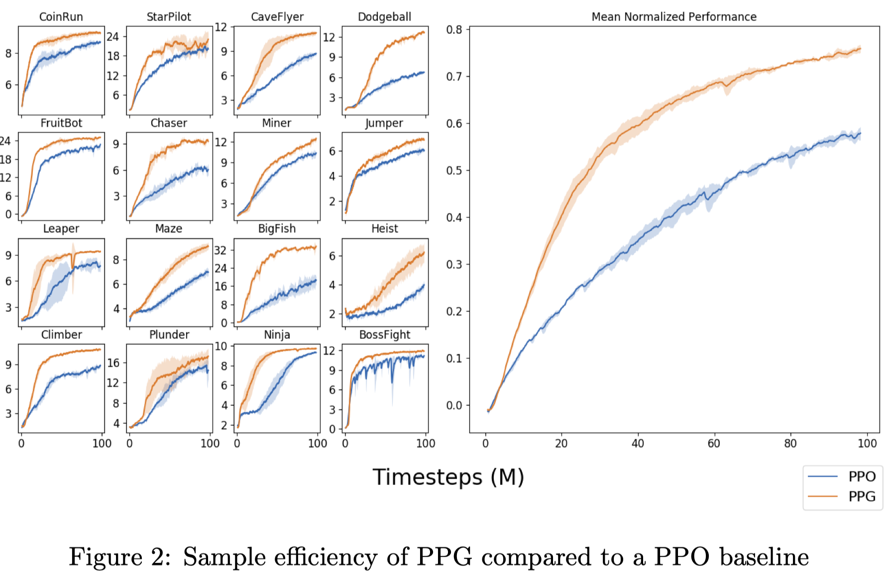
Phasic Policy Gradient
In PPG, training proceeds in two alternating phases: a policy phase, followed by an auxiliary phase. During the policy phase, we optimize the same objective from PPO using two disjoint networks to represent the policy and value function, respectively.
\[\begin{align} \max_\theta \mathcal J(\theta)&=\mathbb E\left[\min\bigl(r_t(\theta)\hat A_t, \mathrm{clip}(r_t(\theta), 1-\epsilon, 1+\epsilon)\hat A_t\bigr)+cH(\pi_\theta(\cdot|s_t))\right]\tag {1}\\\ \min_\phi \mathcal L^{value}(\phi)&=\mathbb E\left[{1\over 2}(V_\phi(s_t)-\hat V_t)^2\right]\tag {2} \end{align}\]where \(r_t(\theta)={\pi_\theta(a_t\vert s_t)\over \pi_{\theta_{old}}(a_t\vert s_t)}\), \(\hat A_t\) and \(\hat V_t\) are computed with GAE, \(\theta\) and \(\phi\) are the parameters of the policy and value networks, respectively. The use of disjoint parameters ensures two objectives do not interfere each other.
In order to retain the benefit of joint training, we train an auxiliary loss during the auxiliary phase. Specifically, we train an additional value head under the constraint of preserving the original policy. This is achieved by the following loss
\[\begin{align} \min_\theta \mathcal L^{joint}(\theta)=\mathbb E_t\left[{1\over 2}(V_\theta(s_t)-\hat V_t)^2\right]+\beta \mathbb E_t[D_{KL}(\pi_{\theta_{old}}(\cdot|s_t)\Vert\pi_\theta(\cdot|s_t))]\tag {3} \end{align}\]where \(\pi_{\theta_{old}}\) is the policy right before the auxiliary phase begins, \(V_\theta\) is an auxiliary value head of the policy network, and \(\hat V_t\) is the same target as the one in Equation \((2)\). The KL term penalizes the deviation of the policy caused by the training of the value function, ensuring that auxiliary training does not corrupt the policy we learned.
Algorithm
The algorithm repeats the following three steps
\[\begin{align} &\mathbf{for}\ phase=1,2,\dots\ \mathbf {do}\\\ &\quad\text{Initialize empty buffer }B\\\ &\quad\mathbf {for}\ iteration=1, 2, \dots, N_\pi\ \mathbf {do}\\\ &\quad\quad\text{Perform rollouts under current policy }\pi\\\ &\quad\quad\text{Compute value function target }\hat V_t\text{ and advantage }\hat A_t\text{ for collected data}\\\ &\quad\quad\mathbf{for}\ epoch=1, 2,\dots,E_\pi\ \mathbf {do}\\\ &\quad\quad\quad \text{Optimize Equation (1) w.r.t. }\theta\\\ &\quad\quad\mathbf{for}\ epoch=1, 2,\dots,E_V\ \mathbf {do}\\\ &\quad\quad\quad \text{Optimize Equation (2) w.r.t. }\phi\\\ &\quad\quad\text{Add data to }B\\\ &\quad\text{Compute and store current policy }\pi_\theta(\cdot|s_t)\text{ and value target } \hat V\text{ for all states }s_t\\\ &\quad\mathbf {for}\ epoch=1, 2, \dots,E_{aux}\ \mathbf {do}\\\ &\quad\quad\text{Optimize Equation (3) w.r.t. }\theta\text{ on data in }B\\\ &\quad\quad\text{Optimize Equation (2) w.r.t. }\phi\text{ on data in }B \end{align}\]Notice that
-
We perform the auxiliary phase every \(N_\pi\) policy iterations with all data collected in between.
-
We minimize Equation \((2)\) in both phases to increase the sample reuse for value function optimization.
Experiments
The following experiments are done on Procgen environment using the hard difficulty setting.
Hyperparameters
Throughout all experiments, the following hyperparameters are used unless otherwise specified.
| Hyperparameter | Value |
|---|---|
| # policy iterations per auxiliary phase \(N_\pi\) | 32 |
| # policy epochs per policy iteration \(E_\pi\) | 1 |
| # value epochs per policy iteration \(E_V\) | 1 |
| # auxliary epochs in auxiliary phase \(E_{aux}\) | 6 |
| \(\beta\) | 1 |
| # mini-batches per auxiliary epoch per \(N_\pi\), \(N_a\) | 16 |
| \(\gamma\) | .999 |
| \(\lambda\) | .95 |
| # time steps per rollout | 256 |
| # mini batches per epoch | 8 |
| Entropy bonus coefficient \(c\) | .01 |
| PPO clip range \(\epsilon\) | .2 |
| Reward normalization? | Yes |
| Learning rate | \(5\times 10^{-4}\) |
| # workers | 4 |
| # environments per worker | 64 |
| Total timesteps | 100M |
| LSTM? | No |
| Frame Stack? | No |
In the auxiliary phase, PPG performs \(N_\pi\times N_a\) updates every epoch. This incurs a significantly computational cost. We empirically find that reducing it to \(N\times N_a\), where \(N<N_\pi\), improves the performance and saves time. Note that we still store all data from the previous \(N_\pi\) policy iterations; taking only the data from the recent \(N\) iterations impairs the performance as it may be more likely to overfit.
Policy Sample Reuse
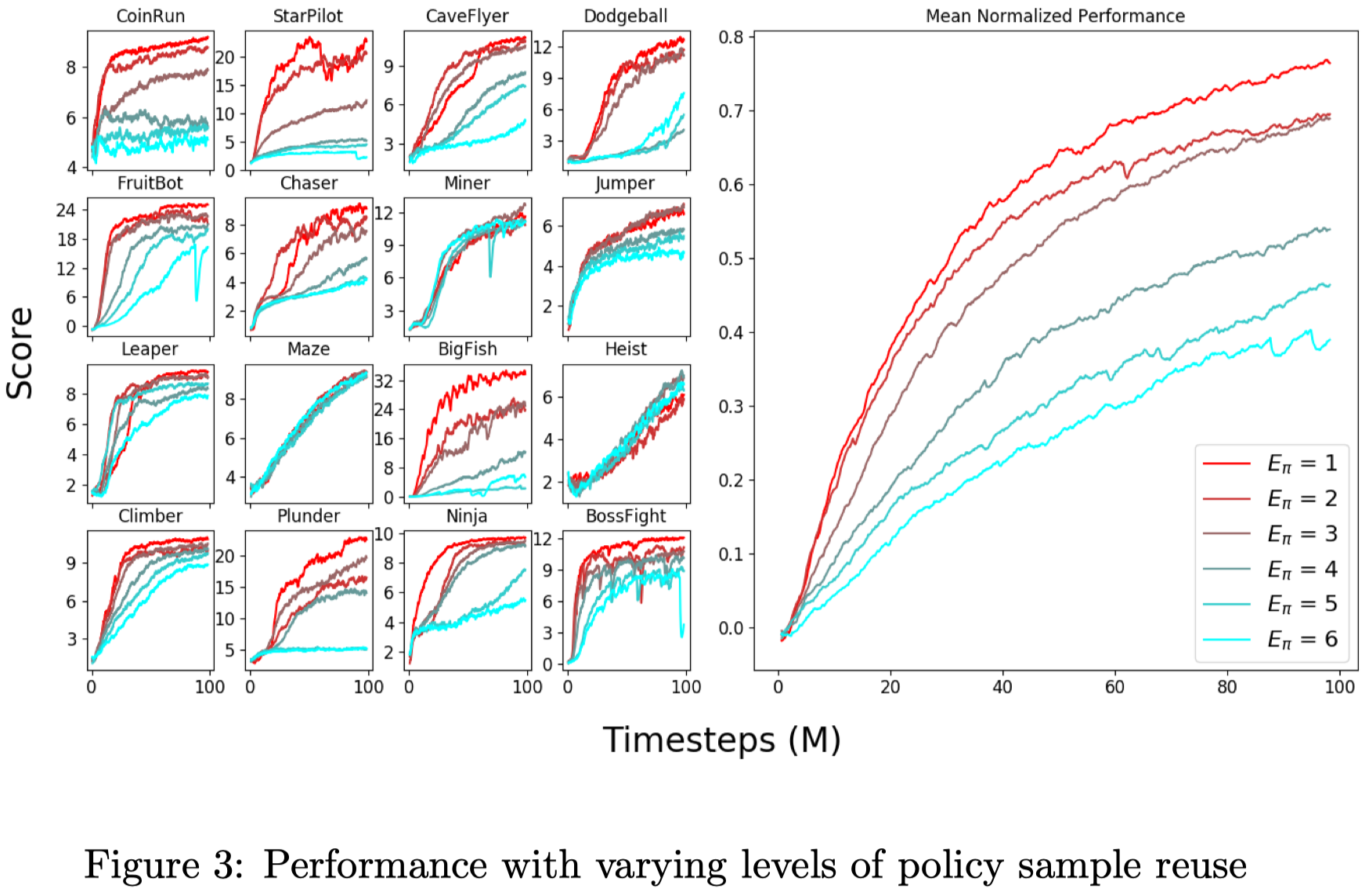
Figure 3 shows that training with a single policy epoch (\(E_\pi=1\)) is almost always optimal in PPG. This suggests that the PPO baseline benefits from greater sample reuse only because the extra epoch offer additional value function training. When value function and policy trainings are properly isolated, we see little benefit from training the policy beyond a single epoch. Of course, various hyperparameters will influence this result. If we use an artificially low learning rate, for instance, it will become advantageous to increase policy sample reuse. Our present conclusion is simply that when using well-tuned hyperparameters, performing a single policy epoch is near-optimal.
Value Sample Reuse
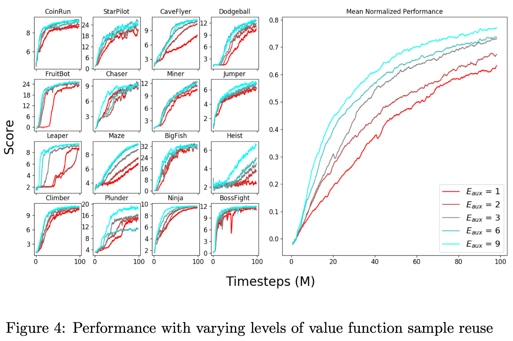
Figure 4 shows that training with additional auxiliary epoch is generally beneficial. This offers two benefits. First, due to the optimization of \(\mathcal L^{joint}\), we may expect better-trained features to be shared with the policy. Second, due to the optimization of \(\mathcal L^{value}\), we may expect to train a more accurate value function, whereby reducing the variance of the policy gradient in future policy phases.
Auxiliary Phase Frequency
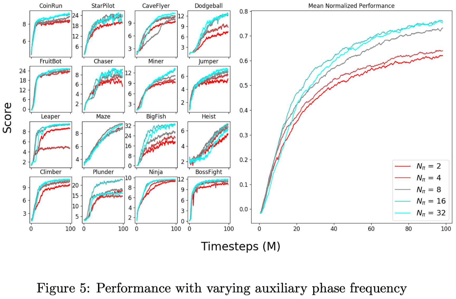
Figure 5 shows that the performance decreases when we perform the auxiliary phase too frequently(\(N_\pi\) is small). Kobbe et al. 2020 conjecture that each auxiliary phase interferes with policy optimization, and that performing frequent auxiliary phases exacerbates this effect.
KL Penalty vs Clipping
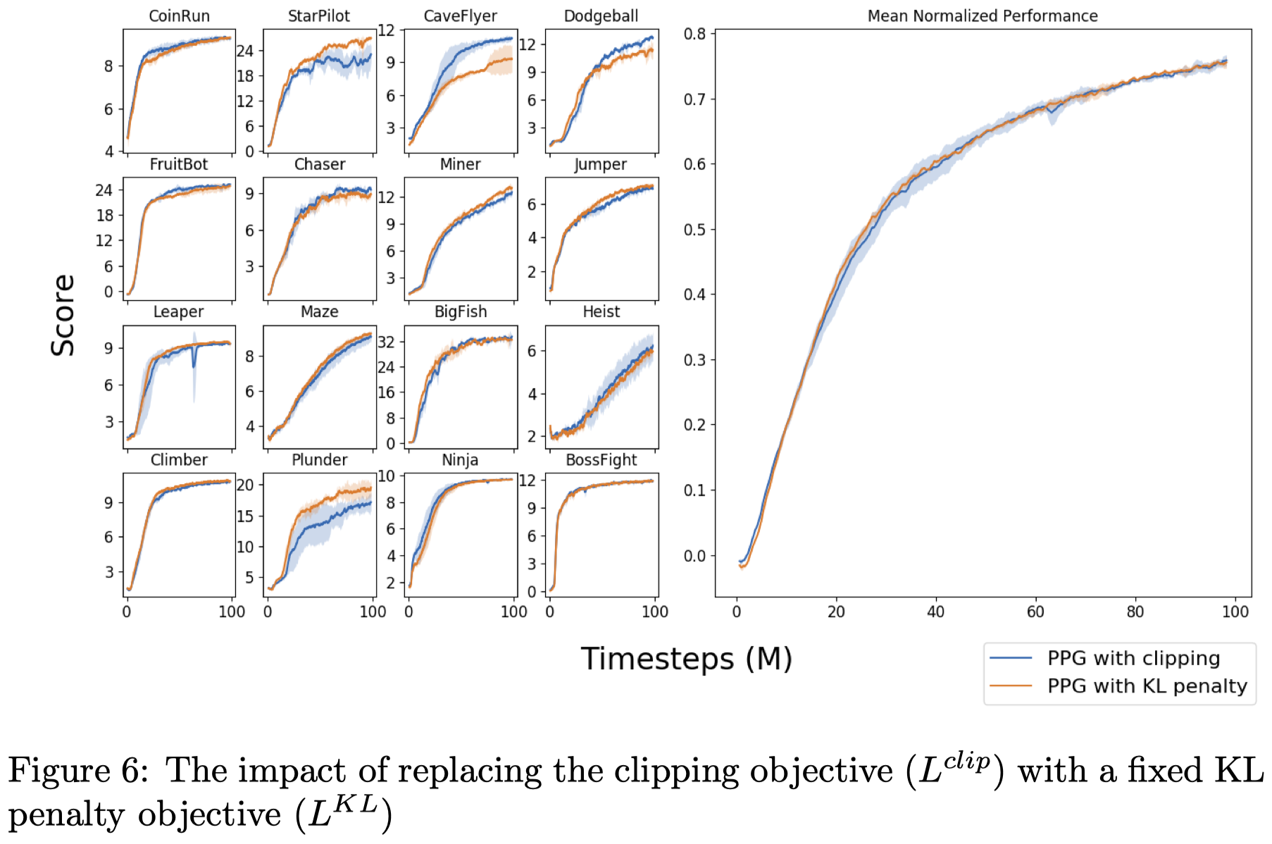
Figure 6 shows that a constant KL penalty (with coefficient \(1\)) on the policy objective yields similar performance as the PPO’s clipping objective. Kobbe et al. 2020 suspect that using clipping (or an adaptive KL penalty) is more important when rewards are poorly scaled. This can be avoided by normalizing rewards so that discounted returns have approximately unit variance.
Single-Network PPG
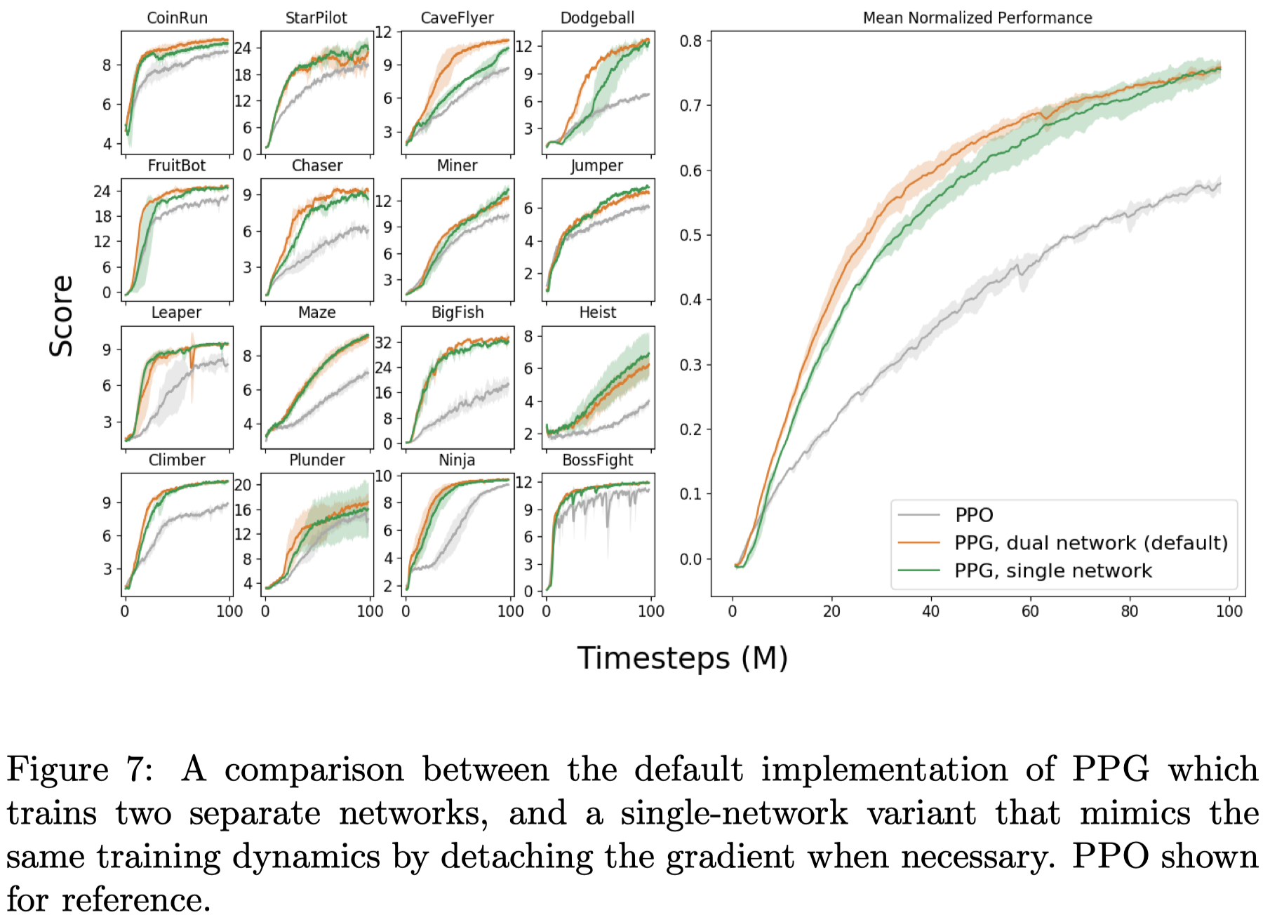
Figure 7 shows that PPG can also be achieved using a single network without losing much performance. This is done by stopping the value gradient at the last shared layer during the policy phase, and taking the value gradient with respect to all parameters during the auxiliary phase. (Blake Wulfe, the winner of the Procgen competition, observed that stopping the value gradient rendered the method unstable in some environments and instead he reduce the value loss coefficient to \(0.25\)).
Shared vs Separate Networks in PPO
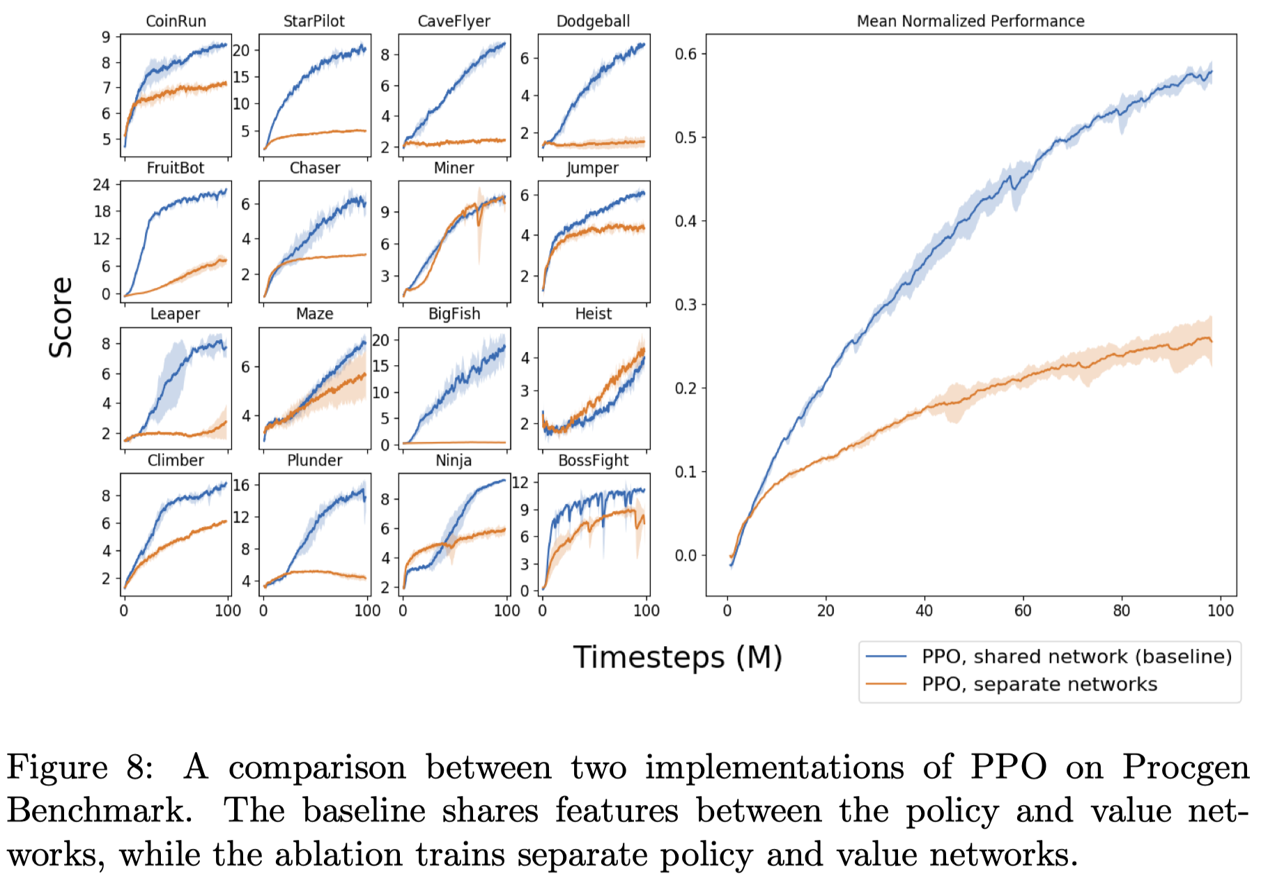
Figure 8 shows that simply separating value from policy network leads to poor performance, indicating constructive benefits of training both policy and value losses jointly.
Auxiliary Phase Value Function Training
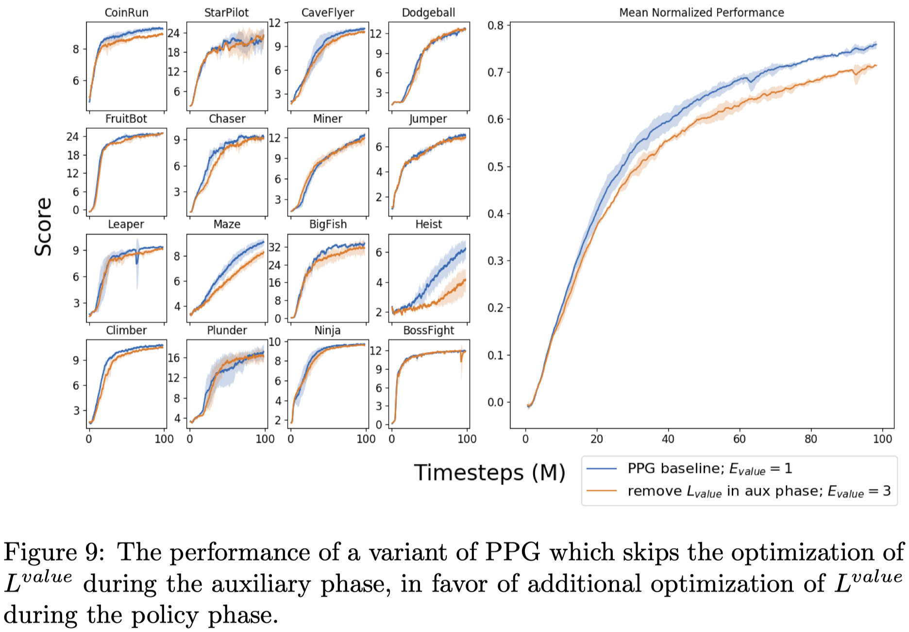
Figure 9. Shows that removing value function training in auxiliary phase and increasing value function training in policy phase achieve comparable results.
References
Cobbe, Karl, Jacob Hilton, Oleg Klimov, and John Schulman. 2020. “Phasic Policy Gradient.” http://arxiv.org/abs/2009.04416.

