
TL; DR
PWIL trains an off-policy algorithm with the reward function defined below
\[\begin{align} r_i=&\alpha\exp(-{\beta T\over\sqrt{|\mathcal S|+|\mathcal A|}}c_i) \end{align}\]where \(c_i\) is the minimum cost of moving \((s^\pi_i,a^\pi_i)\) to some \((s_j^e,a_j^e)\)(s).
Despite PWIL achieves extremely well performance on Mujoco environments, I highly suspect its generality as state discrepancy measure is unreliable when the environment is not static or the initial state varies.
Objective
In order to learn from a few demonstrations, PWIL minimizes the Wasserstein distance between the state-action distribution of the learned policy \(\hat\rho_\pi\) and that of the expert \(\hat\rho_e\) in the trajectory setting
\[\begin{align} \inf_{\pi\in\Pi}\mathcal W_p^p(\hat\rho_\pi,\hat\rho_e)=\inf_{\pi\in\Pi}\inf_{\theta\in\Theta} \sum_{i=1}^T\sum_{j=1}^D d((s_i^\pi,a_i^\pi),(s_j^e,a_j^e))^p\theta[i,j]\tag 1 \end{align}\]where \(\Theta(i,j)\) is the set of all coupling between \(i\) and \(j\), \(d\) is a distance function.
Method
Episodic version
In the context of RL, we compute \(\theta_\pi^*\) as the optimal coupling for the policy \(\pi\):
\[\begin{align} \theta_\pi^\*=\underset{\theta\in\Theta}{\arg\min}\sum_{i=1}^T\sum_{j=1}^D d((s_i^\pi,a_i^\pi),(s_j^e,a_j^e))^p\theta[i,j] \end{align}\]given which we minimize the following cost using an RL method.
\[\begin{align} \inf_{\pi\in\Pi}\mathcal W_1(\hat\rho_\pi,\hat\rho_e)=&\inf_{\pi\in\Pi}\sum_{i=1}^Tc_{i,\pi}^\*\\\ where\quad c^\*_{i,\pi}=&\sum_{j=1}^Dd((s_i^\pi,a_i^\pi),(s_j^e,a_j^e))^p\theta[i,j] \end{align}\]Note that \(c_{i,\pi}^*\) depends on the optimal coupling, which can only be computed at the very end of an episode. This can be problematic if an agent learns in an online manner or in large time-horizon tasks.
Greedy version
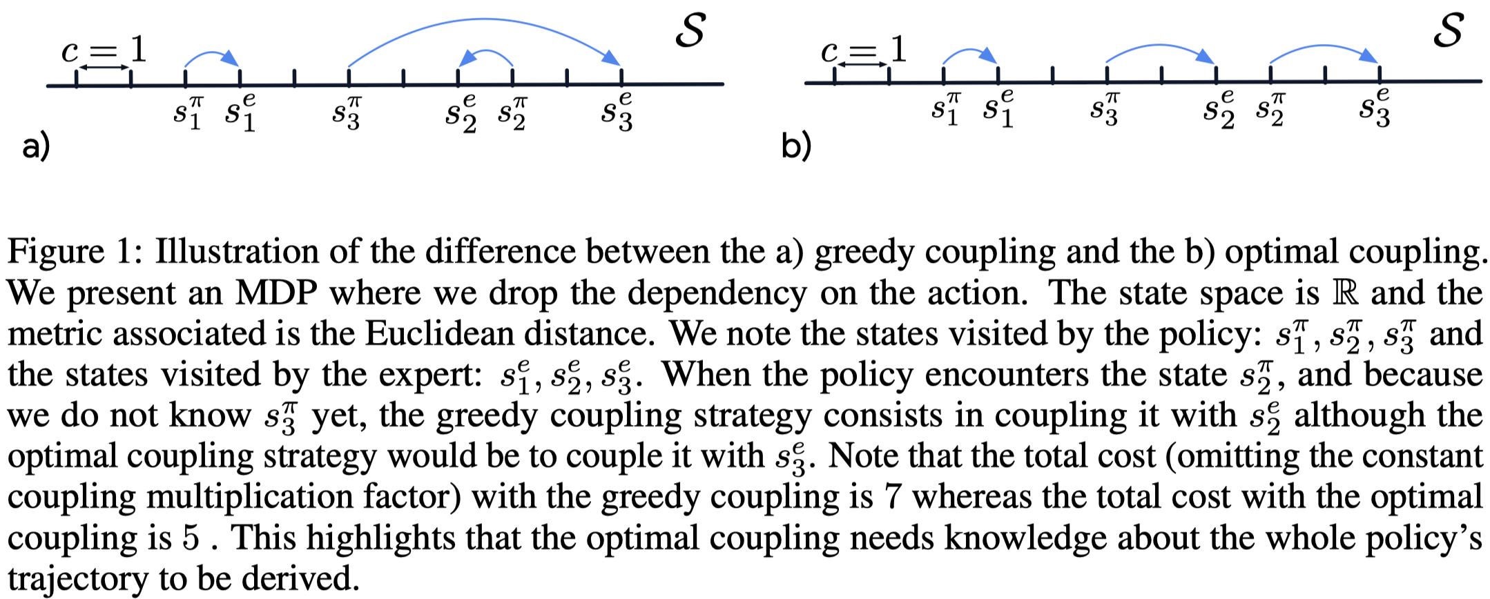
A workaround is to define a greedy coupling \(\theta^g_\pi\in\Theta\) recursively for \(1\le i\le T\) as
\[\begin{align} \theta_\pi^g[i,:]=&\underset{\theta[i,:]\in\Theta_i}{\arg\min}\sum_{j=1}^Dd((s_i^\pi,a_i^\pi), (s_j^e,a_j^e))\theta[i,j]\\\ where\quad\Theta_i=&\Big\{\theta[i,:]\in\mathbb R_+^D\Big\vert\underbrace{\sum_{j=1}^D\theta[i,j]={1\over T}}_{\text{constraint (a)}},\underbrace{\forall k\in[1:D],\sum_{i'=1}^{i-1}\theta_g[i',k]+\theta[i,k]\le{1\over D}}_{\text{constraint(b)}}\Big\} \end{align}\]In the terminology of earth mover’s distance, the constraint \((a)\) means that all the dirt at the \(i^{th}\) timestep needs to be moved, and the constraint \((b)\) constrains the target capacity. The greedy coupling is suboptimal due to the constraint on the target capacity as Figure 1 demonstrates. Although it becomes optimal when the target capacity constraint is removed, it sometimes leads to performance drop as shown in the experimental results.
Now the cost function is defined as
\[\begin{align} c^g_{i,\pi}=\sum_{j=1}^Dd((s_i^\pi,a_i^\pi),(s_j^e,a_j^e))^p\theta^g_\pi[i,j] \end{align}\]Distance and reward functions
For the distance function, PWIL defines the standardized Euclidean distance which is the L2 distance on the concatenation of the observation and the action, weighted along each dimension by the inverse standard deviation of the expert demonstrations.
The reward function should be a decreasing function of the cost. In practice, PWIL defines the reward function as
\[\begin{align} r_i=\alpha\exp(-{\beta T\over\sqrt{|\mathcal S|+|\mathcal A|}}c_i) \end{align}\]where \(\alpha=5\) and \(\beta=5\) is used in the experiments. The scaling factor \(T\over\sqrt{\vert \mathcal S\vert +\vert \mathcal A\vert }\) acts as a normalizer on the dimensionality of the state and action spaces and on the time horizon of the task.
Algorithm
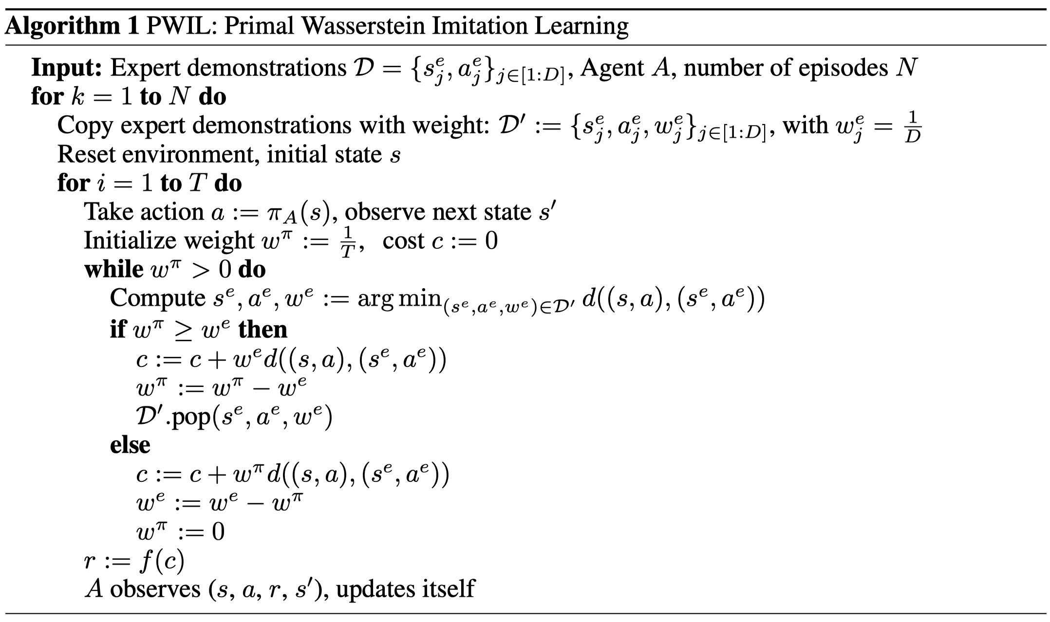
Note the runtime of a single reward step computation is \(\mathcal O((\vert \mathcal S\vert +\vert \mathcal A\vert )D+{D^2\over T})\), where \(\mathcal O((\vert \mathcal S\vert +\vert \mathcal A\vert )D)\) is used for computing all \(d((s,a),(s^e,a^2))\) at once and \(\mathcal O({D^2\over T})\) is for the while loop.
Experimental Results
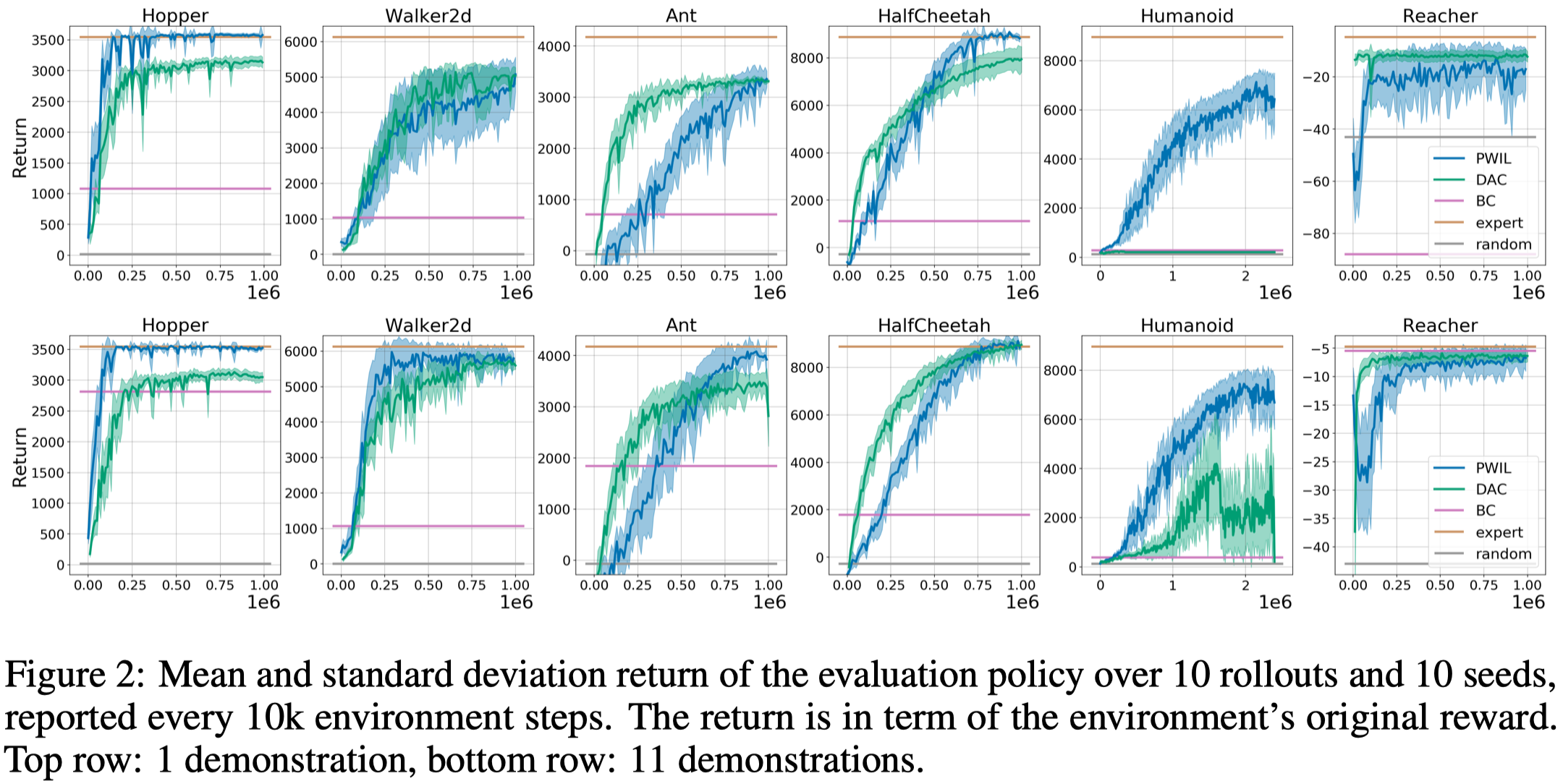
Figure 2 compares PWIL with DAC and BC. Note that PWIL is able to learn from a single demonstration for challenging tasks such as Humanoid.
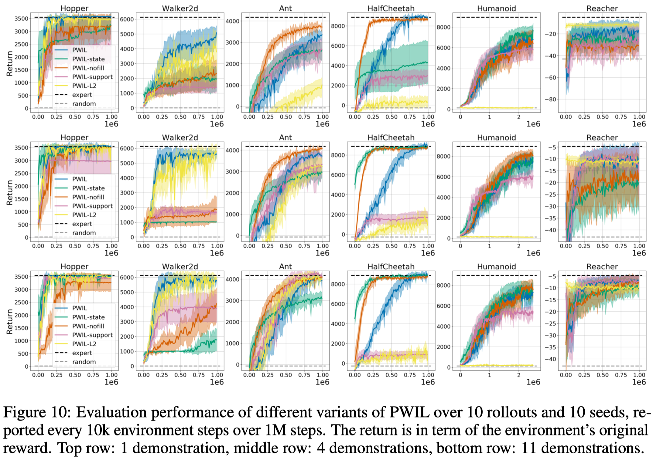
Figure 10 demonstrates the result of the ablation study, where
- PWIL-state does not use the expert’s actions.This leads to a huge performance drop in Walker2d while leave the other almost the same.
- PWIL-nofill does not prefill the replay buffer with expert transitions. This leads to a drop in performance in most games, especially for Walker
- PWIL-L2 uses the simple L2 distance without normalization. This results in a significant drop in all environments except for Hopper and Walker2d
- PWIL-support does not constrain the target capacity. In other words, we no longer have the while loop in the algorithm. This leads to a significant drop in Walker2d and a slight drop in Hopper.
References
Dadashi, Robert, Léonard Hussenot, Matthieu Geist, and Olivier Pietquin. 2020. “Primal Wasserstein Imitation Learning.” ArXiv, 1–19.