
Introduction
In multi-agent environments, one way to accelerate the coordination effect is to enable multiple agents to communicate with each other in a distributed manner and behave as a group. In this post, we discuss a multi-agent reinforcement learning framework, called SchedNet proposed by Kim et al., in which agents learn how to schedule communication, how to encode messages, how to act upon received messages.
It is worth noting that Kim et al. comment
SchedNet is not intended for competing with other algorithms for cooperative multi-agent tasks without considering scheduling, but a complementary one.
Problem Setting
We consider multi-agent scenarios wherein the task at hand is of a cooperative nature and agents are situated in a partially observable environment. We formulate such scenarios into a multi-agent sequential decision-making problem, such that all agents share the goal of maximizing the same discounted sum of rewards. As we rely on a method to schedule communication between agents, we impose two restrictions on medium access:
- Bandwidth constraint: The agent can only pass \(L\) bits message to the medium every time.
- Contention constraint: The agents share the communication medium so that only \(K\) out of \(n\) agents can broadcast their messages.
We now formalize MARL using DEC-POMDP(DECentralized Partially Observable Markov Decision Process), a generalization of MDP to allow a distributed control by multiple agents who may be incapable of observing the global state. We describe a DEC-POMDP by a tuple \(<\mathcal S, \mathcal A, r, P, \Omega, \mathcal O, \gamma>\), where:
- \(s\in\mathcal S\) is the environment state, which is not available to agents,
- \(a_i\in\mathcal A\) and \(o_i\in \Omega\) are the action and observation for agent \(i\in\mathcal N\)
- \(r:\mathcal S\times \mathcal A^N\mapsto \mathbb R\) is the reward function shared with all agents
- \(P: \mathcal S\times \mathcal A^N\mapsto \mathcal S\) is the transition function
- \(\mathcal O:\mathcal S\times \mathcal N\mapsto \Omega\) is the emission/observation probability
- \(\gamma\) denotes the discount factor
SchedNet
Overview
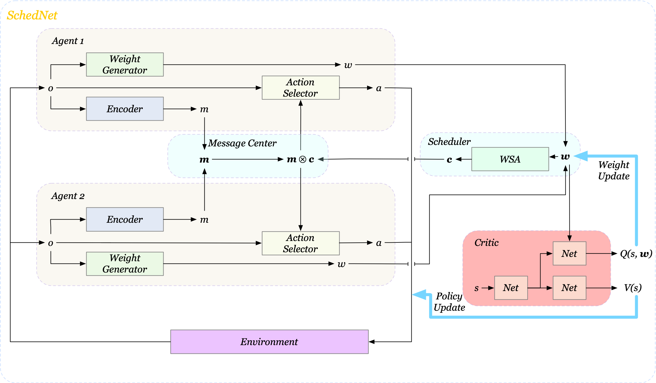
Before diving into details, we first take a quick look at the architecture(Figure1) to get an overview of what’s going on here. At each time step, each agent receives its observation, and pass the observation to a weight generator and an encoder to produce a weight value \(w\) and a message \(m\), respectively. All weight values are then transferred to a central scheduler, which determines which agents’ messages are scheduled to broadcast via a schedule vector \(\mathbf c=[c_i]_n, c_i\in{0, 1}\). The message center aggregates all messages along with the schedule vector \(\mathbf c\) and then broadcasts selected messages to all agents. At last, each agent takes an action based on these messages and their observations.
As we will see next, SchedNet trains all its components through the critic, following the centralized training and distributed execution framework.
Weight Generator
The weight generator takes observation as input and outputs a weight value which is then used by the scheduler to schedule messages. We train the weight generator through the critic by maximizing \(Q(s,\mathbf w)\), an action-value function. To get a better sense of what’s going on here, let’s take the weight generator as a deterministic policy network, and absorb all other parts except the critic into the environment. Then the weight generator and critic will form a DDPG structure. In this setup, the weight generator is responsible for answering the question: “what weight I generate could maximize the environment rewards from here on?”. As a result, we have the following objective
\[\begin{align} \mathcal L(Q)&=\min_Q\mathbb E_{s,a_{1:N}, s',\mathbf w, \mathbf w'\sim\mathcal D}\left[\big(r(s,a_{1:N})+\gamma Q(s',\mathbf w')-Q(s,\mathbf w)\big)^2\right]\\\ \mathcal J(WG)&= \max_{\mathbf{WG}}\mathbb E_{s, \mathbf o\sim \mathcal D}\left[Q(s, \mathbf {WG}(\mathbf o))\right] \end{align}\]where we use bold-face fonts to highlight aggregate notations of multiple agents as we did in Figure.1. It is essential to distinguish \(s\) from \(o\); \(s\) is the environment state, while \(o\) is the observation from the viewpoint of each agent. This simplifies the learning process. More importantly, it is theoretically not sound(albeit it may work in practice) to take observations as the critic input since the critic is updated based on the Bellman equation, which is built upon the Markov property.
Scheduler
Back when we described the problem setting, two constraints were imposed on the communication process. The bandwidth limitation \(L\) can easily be implemented by restricting the size of message \(m\). We now focus on imposing \(K\) on the scheduling part.
The scheduler adopts a simply weight-based algorithm, called WSA(Weight-based Scheduling Algorithm), to select \(K\) agents. Two proposals are considered in the paper:
- \(Top(k)\): Selecting top \(k\) agents in terms of their weight values
- \(Softmax(k)\): Computing softmax values \(\sigma_i(\mathbf w)={e^{w_i}\over\sum_{j=1}^ne^{w_j}}\) for each agent \(i\), and then randomly selecting \(k\) agents according to this softmax values.
The WSA module outputs a schedule vector \(\mathbf c=[c_i]_n, c_i\in{0, 1}\), where each \(c_i\) determines whether the agent \(i\)’s message is scheduled to broadcast or not.
As a side note: the official implementation takes the concatenation of the observation and the moving average schedule as the observation of predators.
Message Encoder, Message Center, and action selector
The message encoder encodes observations to produce a message \(m\). The message center aggregates all messages \(\mathbf m\), and selects which messages to broadcast based on \(\mathbf c\). The resulting message \(\mathbf m\otimes\mathbf c\) is the concatenation of all selected message. For example, for \(\mathbf m=[000, 010, 111]\) and \(\mathbf c=[101]\), the final message to broadcast is \(\mathbf m\otimes\mathbf c=[000111]\). Each agent’s action selector then chooses an action based on this message and its own observation.
We train the message encoders and action selectors via an on-policy algorithm, with the state-value function \(V(s)\) in the critic. The gradient of its objective is
\[\begin{align} \nabla_\pi J(\pi)=\mathbb E_{s,a,o\sim\pi(\tau)}[\nabla_{\pi}\log\pi(a|o,\mathbf m\otimes\mathbf c)(r(s,a)+\gamma V(s')-V(s))] \end{align}\]where \(\pi\) denotes the aggregate network of the encoder and selector, and \(V\) is trained with the following objective
\[\begin{align} \mathcal L(V)=\mathbb E_{s,a\sim\pi(\tau)}\left[(r(s,a)+\gamma V(s')-V(s))^2\right] \end{align}\]Discussion
Two Different Training Procedure?
The authors train the weight generators and action selectors using different methods but with the same data source. Specifically, they train the weight generators using a deterministic policy-gradient algorithm(an off-policy method), while simultaneously training the action selectors using a stochastic policy-gradient algorithm(an on-policy method). This could be problematic in practice since the stochastic policy-gradient method could diverge under the training with off-policy data. The official implementation ameliorates this problem using a small replay buffer of \(10^4\) transitions, which, however, may impair the performance of weight generator training.
We could bypass this problem by reparameterizing the critic such that it takes as inputs state \(s\) and actions \(a_1,a_2,\dots\) and outputs the corresponding \(Q\)-value. In this way, we make both trained with off-policy methods. Another conceivable way is to separate the training process from environment interaction if one insists on stochastic policy-gradient methods. Note that it is not enough to simply separate the policy training since the update of the weight generator could change the environment state distribution.
Same message weights?
As shown in Figure.1, all agents receive the same message \(\mathbf m\otimes\mathbf c\). This may not be desirable in some cases since different agent may benefit from different messages. One may replace WSA with a variant of exemplary network to learn specific information for each agent. As some food for thought, the following model gives an example:
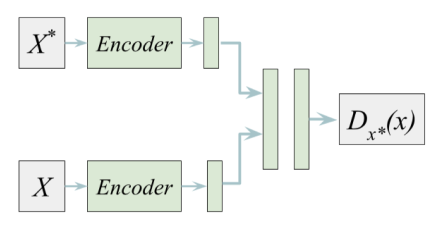
where \(X^*\) is the input(e.g. weights in Figure 1) from the target agent that the message center will send message to, \(X\) are inputs from other agents. \(D_{x^*}(x)\) computes the desire weight of message \(X\) to \(X^*\).
References
Daewoo Kim, Moon Sangwoo, Hostallero David, Wan Ju Kang, Lee Taeyoung, Son Kyunghwan, and Yi Yung. 2019. “Learning To Schedule Communication In Multi-Agent Reinforcement Learning.” ICLR, 1–17.