
Preliminaries
\(q\)-Exponential, \(q\)-Logarithm, and Tsallis Entropy
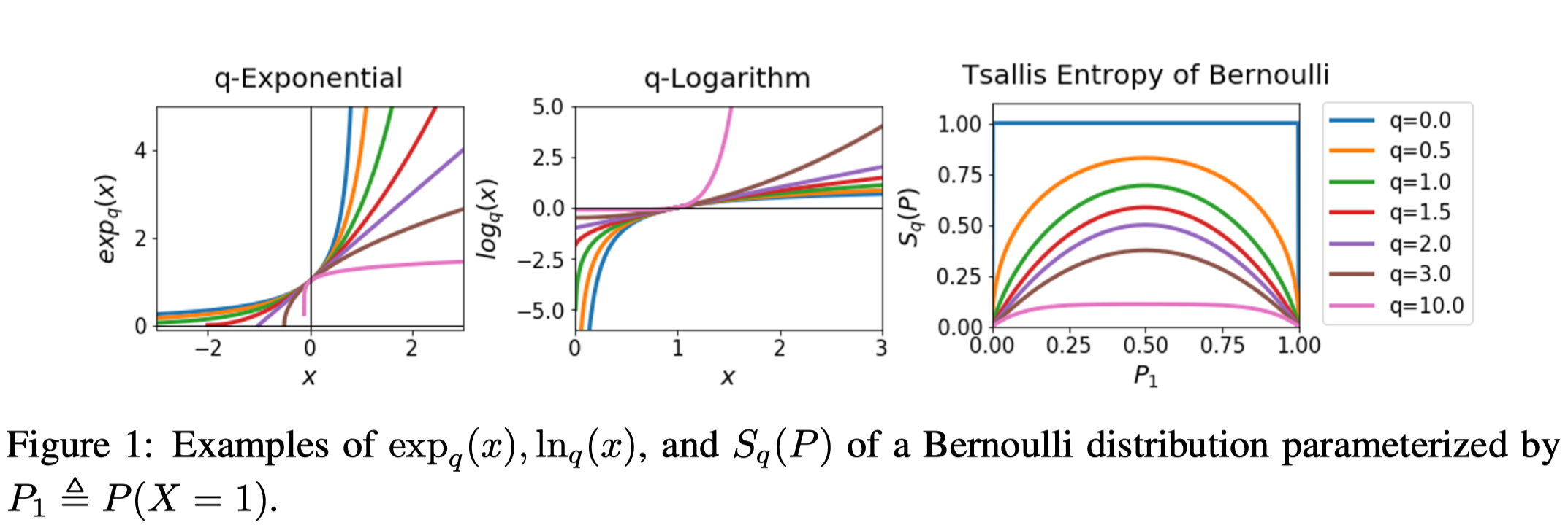
\(q\)-exponential and \(q\)-logarithm are defined as follows:
\[\begin{align} \exp_q(x):=&\begin{cases} \exp(x),&\text{if }q=1\\\ [1+(q-1)(x)]_+^{1\over q-1}&\text{if }q\ne 1 \end{cases}\tag 1\\\ \log_q(x):=&\begin{cases} \log(x)&\text{if }q=1\text{ and }x>0\\\ {x^{q-1}-1\over q-1}&\text{if }q\ne 1\text{ and }x>0 \end{cases}\tag 2 \end{align}\]where \([x]_+=\max(x,0)\) and \(q\) is a real number.
Note that
- \(\forall x> 0, \exp_q(\log_q(x))=x\) and \(\forall \exp_q(x)\ge 0, \log_q(\exp_q(x))=x\).
- \(\log_q(x)\) is non-decreasing w.r.t. \(q\) as its derivative are non-negative.
- These are different from the original ones in Amari et al. 2011 but we can recover the original ones by setting \(q=2-q’\).
The property of \(q\)-exponential and \(q\)-logarithm depends on the value of \(q\). We’d like to note that, for all \(q\), \(\log_q(x)\) is a monotonically increasing function w.r.t. \(x\). However, the tendencies of their gradients are different. For \(q>2\), \(d\log_q(x)/dx\) is an increasing function, while, for \(q<2\), \(d\log_q(x)/dx\) is a decreasing function. Especially, when \(q=2\), the gradient becomes a constant. This property will play an important role for controlling the exploration-exploitation trade-off when we model a policy using parameterized function approximation.
The Tsallis entropy of a random variable \(X\) with distribution \(P\) is defined as follows(Amari et al. 2011)
\[\begin{align} S_q(P):=\mathbb E_{x\sim P}[-\log_q(P(x))]\tag 3 \end{align}\]Here, \(q\) is called an entropic-index.
The Tsallis entropy can represent various types of entropy by varying the entropic index \(q\). For example, when \(q=1\), \(S_1(P)\) becomes the Shannon entropy and when \(q=2\), \(S_2(P)\) becomes the sparse Tsallis entropy. Furthermore, when \(q\rightarrow \infty\), \(S_q(P)\) converges to zero.
\(q\)-maximum
For a function \(f(x)\), \(q\)-maximum is defined as follows
\[\begin{align} q\text-\max_x(f(x))=\max_{P}\left[\mathbb E_{x\sim P}[f(x)]+S_q(P)\right] \end{align}\]Theorem 1 shows \(q\)-maximum bounds the maximum of \(f(x)\).
Theorem 1. For any function \(f(x)\) defined on a finite input space \(\mathcal X\), the \(q\)-maximum satisfies the following inequalities
\[\begin{align} q\text-\max_x(f(x))+\log_q(1/|\mathcal X|)\le \max_x(f(x))\le q\text-\max_x(f(x)) \end{align}\]Proof. The upper bound is given since \(S_q(P)\) is non-negative. The lower bound is derived as follows
\[\begin{align} q\text-\max_x(f(x))=&\max_{P}\left[\mathbb E_{x\sim P}[f(x)]+S_q(P)\right]\\\ \le&\max_P\mathbb E_{x\sim P}[f(x)]+\max_P S_q(P)\\\ =&\max_P\mathbb E_{x\sim P}[f(x)]-\log_q(1/|\mathcal X|) \end{align}\]where the last equality is obtained because \(S_q(P)\) has the maximum at an uniform distribution.
Maximum Tsallis Entropy RL
We formulate the objective of the maximum Tsallis entropy RL
\[\begin{align} \max_\pi\mathcal J_q(\pi)=\mathbb E_{\pi}\left[\sum_{t}\gamma \big(r(s_t,a_t)+\alpha S_q(\pi_t)\big)\right]\tag 4 \end{align}\]The corresponding state and action value functions are defined as follows
\[\begin{align} V_q^\pi(s_t)=&\mathbb E_{\pi}\left[\sum_{t}\gamma \big(r_t+\alpha S_q(\pi_t)\big)\right]\\\ =&\mathbb E_\pi[Q_q^\pi(s_t,a_t)]+\alpha S_q(\pi_t)\\\ Q_q^\pi(s_t,a_t)=&r_t+\gamma \mathbb E_{s_{t+1}}[V_q^\pi(s_{t+1})] \end{align}\]We can also derive the Tsallis Bellman optimality equations
\[\begin{align} V_q^\*(s_t)=&q\text-\max_a Q_q^\*(s,a)\\\ =&\max_\pi \mathbb E_\pi[Q_q^\*(s_t,a_t)]+\alpha S_q(\pi_t) \tag 5\\\ Q_q^\*(s_t,a_t)=&r_t+\gamma \mathbb E_{s_{t+1}}[V_q^\*(s_{t+1})]\tag 6\\\ \pi_q^\*(a_t|s_t)=&{1\over Z}\exp_q(Q_q^\*(s_t,a_t)/\alpha q)\tag 7 \end{align}\]Proof. We prove Equation \((7)\) from Equation \((5)\). First, we add policy constraints and rewrite Equation \((5)\) as a constraint optimization problem
\[\begin{align} \max_\pi \mathbb E_\pi[Q_q^\*(s,a)]&+\alpha S_q(\pi)\quad\forall s\sim d(s)\\\ s.t.\quad\sum_a\pi(a|s)=&1\\\ \pi(a|s_t)\ge &0 \end{align}\]The generalized Lagrangian is
\[\begin{align} \mathcal L(\pi,\lambda,\nu)=\sum_sd(s)\left(\sum_a\pi(a|s)\big(Q_q^\*(s,a)+\alpha \log_q(\pi(a|s)\big)-\lambda(s)(\sum_a\pi(a|s)-1)-\sum_a\nu(a|s)\pi(a|s)\right) \end{align}\]Setting the first-order derivative of \(\mathcal L\) w.r.t. \(\pi(a_t\vert s_t)\) to zero, we have
\[\begin{align} {\partial\over \partial\pi(a|s)}\mathcal L(\pi,\lambda,\nu)=&0\\\ Q^\*(s,a)-\alpha{\pi(a|s)^{q-1}-1\over q-1}-\alpha\pi(a|s)^{q-1}-\lambda(s)-\nu(a|s)=&0\\\ Q^\*(s,a)-\alpha{q\pi(a|s)^{q-1}-1\over q-1}-\lambda(s)-\nu(a|s)=&0\\\ Q^\*(s,a)-\alpha{q(\pi(a|s)^{q-1}-1)+q-1\over q-1}-\lambda(s)-\nu(a|s)=&0\\\ Q^\*(s,a)-\alpha (q\log_q\pi(a|s)-1)-\lambda(s)-\nu(a|s)=&0\\\ \log_q\pi(a|s)=&{Q^\*(s,a)-\lambda(s)-\nu(a|s)+\alpha\over \alpha q}\\\ &\quad\color{red}{\mu(s)={\lambda(s)-\alpha\over \alpha q}}\\\ \pi(a|s)=&\exp_q({Q^\*(s,a)/ \alpha q-\mu(s)}) \end{align}\]where the last step is feasible as \(\nu(a\vert s)\) is zero for actions with positive probabilities; for any zero-probability action, (hmmm, not today.)
Also note that the second-order derivative of \(\mathcal L\) w.r.t. \(\pi(a_t\vert s_t)\) is alway negative:
\[\begin{align} {\partial^2\over \partial\pi(a_t|s_t)^2} \mathcal L(\pi,\lambda,\nu)=-\alpha q\pi(a_t|s_t)^{q-2}<0 \end{align}\]Therefore \(\mathcal L\) is concave and Equation \((7)\) gives the optimal policy.
Performance Error Bounds
Theorem 2. bounds the performance error of a Tsallis MDP.
Theorem 2. Let \(\mathcal J(\pi)\) be the expected sum of rewards of a given policy, \(\pi^*\) be the optimal policy of the original MDP, and \(\pi^*_q\) be the optimal policy of a Tsallis MDP with an entropic index \(q\). Then, the following inequality holds
\[\begin{align} \mathcal J(\pi^\*)+\alpha(1-\gamma)^{-1}\log_q(1/|\mathcal A|)\le \mathcal J(\pi_q^\*)\le J(\pi^\*) \end{align}\]where \(\vert \mathcal A\vert \) is the cardinality of \(\mathcal A\) and \(q > 0\).
Proof. The upper bound is derived by the definition of \(\pi^*\). In the rest of the proof, we derive the lower bound.
We first rewrite Equation \((4)\) as follows
\[\begin{align} \mathcal J_q(\pi)=\mathcal J(\pi)+\alpha\sum_{t}\gamma^tS_q(\pi_t) \end{align}\]From which we derive the upper bound for the optimal policy
\[\begin{align} \mathcal J(\pi^\*)\le& \mathcal J_q(\pi_q^\*)\\\ =&\mathcal J(\pi_q^\*)+\alpha\sum_{t}\gamma^tS_q(\pi_t^\*)\\\ \le&\mathcal J(\pi_q^\*)+\alpha\sum_{t}\gamma^t\max_{\pi_t}S_q(\pi_t^\*)\\\ =&\mathcal J(\pi_q^\*)-\alpha\sum_{t}\gamma^t\log_q(1/|\mathcal A|)\\\ =&\mathcal J(\pi_q^\*)-\alpha(1-\gamma)^{-1}\log_q(1/|\mathcal A|) \end{align}\]where the first step holds because \(S_q(\pi)\) is non-negative. This gives us the lower bound of \(\mathcal J(\pi_q^*)\).
Although a large value of \(q\) gives a tighter lower bound, it also leads to less exploration and thus premature convergence. In practice, \(q\in[1,2]\) is observed to work best. Also notice that \(\alpha\) shows a similar trend to \(q\); a large value of \(\alpha\) relaxes the lower bound while encouraging exploration.
References
Lee, Kyungjae, Sungyub Kim, Sungbin Lim, Sungjoon Choi, and Songhwai Oh. 2019. “Tsallis Reinforcement Learning: A Unified Framework for Maximum Entropy Reinforcement Learning.” ArXiv.
Amari, Shun Ichi, and Atsumi Ohara. 2011. “Geometry of Q-Exponential Family of Probability Distributions.” Entropy 13 (6): 1170–85. https://doi.org/10.3390/e13061170.