
Introduction
Besides algorithmic choices, one way to improve sample efficiency in reinforcement learning is to inject prior knowledge about the structure of the world. This can be done in multiple ways: For example, Vinyals et al. 2019 learns from expert demonstrations a latent variable that takes on a certain type of information and use that to constrain the space of the solution. In this post, we discuss the work of Tirumala et al. 2020, which learns behavior priors that capture the movement and interaction pattern of the agent from a set of related tasks and follow the probabilistic graphic model to regularize the task-specific policies. Experiments show that a good behavior prior can guide exploration, helping escape local optima and improving performance.
TL; DR
-
With an appropriate prior, KL regularized RL provides a meaningful way to explore and boost learning.
-
Information asymmetric is important in KL regularized RL; excessive information hinders the agent’s ability to learn new tasks while too little information yields a meaningless prior.
-
To deal with complex situations, where the prior is multi-modal, we employ the latent variable model and derive the following upper bound for the KL divergence between the current and prior policies:
which can be used in the KL regularized objective
KL-Regularized RL
We consider the KL regularized objective:
\[\begin{align} \mathcal J=\sum_{t}\mathbb E_{ \pi}\left[\gamma^tr(s_t,a_t)-\gamma^tD_{KL}(\pi(a_t|x_t)\Vert \pi_0(a_t|x_t))\right]\tag 1 \end{align}\]where \(r\) is the reward function, \(\pi\) is the policy to learn and \(\pi_0\) is a behavior prior. We also distinguish state from observations: \(s_t\) denotes state at time \(t\) and \(x_t\) the observations, optionally plus actions and rewards, up to time \(t\). It is worth to keep in mind that we usually weight the KL term by a temperature \(\alpha\) to avoid excessive attention focused on the KL term. We omit it throughout this post to keep simplicity. In the rest of the post, we consider to learn a meaningful \(\pi_0\) that provides structured prior knowledge of the environment.
Multi-Task RL
Consider the KL-regularized objective in multi-task setting, where \(\pi_0\) is shared across tasks:
\[\begin{align} \mathcal J=\sum_w\sum_{t}\mathbb E_{\pi}\left[\gamma^tr(s_t,a_t)-\gamma^tD_{KL}(\pi(a_t|x_t)\Vert \pi_0(a_t|x_t))\right]\tag 2 \end{align}\]For a given \(\pi_0\) and task \(w\), it’s easy to derive the optimal policy \(\pi_w\) and values as follows:
\[\begin{align} \pi^\*_w(a|x_t)&=\pi_0(a|x_t)\exp(Q_w^\*(x_t,a)-V_w^\*(x_t))\tag 3\\\ Q_w^\*(x_t,a)&=r(s_t,a)+\gamma\mathbb E_{x_{t+1}\sim P}[V_w^\*(x_{t+1})]\tag 4\\\ \quad V_w^\*(x_t)&=\max_\pi\mathbb E_{a\sim\pi}[Q(x_t,a)-D_{KL}(\pi(a|x_t)\Vert\pi_0(a|x_t))]\tag 5 \end{align}\]On the other hand, given a set of task specific policies, the optimal prior is given by
\[\begin{align} \pi_0^\*(a|x_t)&=\arg\min_\pi\sum_w p(w)D_{KL}(\pi_w\Vert\pi_0)\tag 6\\\ &=\sum_w p(w|x_t)\pi_w^\*(a_t|x_t)\tag 7 \end{align}\]Intuitions: Equation \((3)\) suggests that, given a prior \(\pi_0\), the optimal task-specific policy \(\pi_w^*\) is obtained by reweighing the prior behavior with a term proportional to the soft advantage associated with task \(w\) (or the other way around). In contrast, Equation \((7)\) says the optimal prior \(\pi_0^*\) for a set of task-specific experts \(\pi_w^*\) is the weighted mixture of these task-specific policies, where the weighting is given by the posterior probability of each of these tasks given \(x_t\).
Information Asymmetry for Behavior Priors
A good behavior prior can simplify the learning problem by effectively restricting the search space to a meaningful region. Such priors exhibit structured behaviors, such as gaits and movements of a robot, that exploits the dynamics of the environment with little or no task-specific details. One way to learn such priors is to limit the information they have access to. For example, we can split \(x\) into two disjoint subsets \(x^G\) and \(x^D\)—the former contains all task-specific information while the latter contains the task-agnostic information—and allow \(\pi_0\) access only to \(x^D\). This turns Equation \((1)\) into the following objective
\[\begin{align} \mathcal J=\sum_{t}\mathbb E_{ \pi}\left[\gamma^tr(s_t,a_t)-\gamma^tD_{KL}(\pi(a_t|x_t)\Vert \pi_0(a_t|x_t^D))\right]\tag 8 \end{align}\]It’s worth stressing that the information in \(x^D\) can greatly affect the agent’s learning ability and it’s not as simple as the more the better or the less the better. Excessive information in \(x^D\) may result in a task-specific prior, hindering the agent’s ability to learn in a new task. On the other hand, too little information in \(x^D\) can yield a meaningless prior and the small penalty introduced by the KL term may consume the agent’s will to live. An idea \(x^D\) may just contain enough information shared across all tasks.
Information Bottleneck
Equation \((8)\) also provides an alternative view from information bottleneck:
\[\begin{align} \mathcal J_I=\sum_{t}\mathbb E_{ \pi}\left[\gamma^tr(s_t,a_t)-\gamma^tI(x_t^G,a_t|x_t^D)\right]\tag 9 \end{align}\]Proof: We demonstrate that \(I(x_t^G,a_t\vert x_t^D)=\mathbb E_\pi[D_{KL}(\pi(a_t\vert x_t)\Vert \pi(a_t\vert x_t^D))]\le \mathbb E_\pi[D_{KL}(\pi(a_t\vert x_t)\Vert \pi_0(a_t\vert x_t^D))]\)
\[\begin{align} I(x_t^G,a_t|x_t^D)=&\int\pi(x_t^G,a_t|x_t^D)\log{\pi(x_t^G,a_t|x_t^D)\over\pi(x_t^G|x_t^D)\pi(a_t|x_t^D)}\\\ =&\int\pi(x_t^G,a_t|x_t^D)\log{\pi(a_t|x_t^G,x_t^D)\over\pi(a_t|x_t^D)}=\mathbb E_{\pi}[D_{KL}(\pi(a_t|x_t)\Vert \pi(a_t|x_t^D))]\\\ &\qquad \color{red}{\int\pi(x_t^G,a_t|x_t^D)\log{\pi(a_t|x_t^D)\over\pi_0(a_t|x_t^D)}=\int\pi(x^G|a_t,x_t^D)D_{KL}(\pi(a_t|x_t^D)\Vert\pi_0(a_t|x_t^D))\ge 0}\\\ &\le\int \pi(x_t^G,a_t|x_t^D)\left(\log{\pi(a_t|x_t^G,x_t^D)\over\pi(a_t|x_t^D)}+\log{\pi(a_t|x_t^D)\over\pi_0(a_t|x_t^D)}\right)\\\ &= \mathbb E_{\pi}[D_{KL}(\pi(a_t|x_t)\Vert \pi_0(a_t|x_t^D))] \end{align}\]Because \(I(x_t^G,a_t\vert x_t^D)\le \mathbb E_\pi[D_{KL}(\pi(a_t\vert x_t)\Vert \pi_0(a_t\vert x_t^D))]\), Equation \((9)\) is an upper bound of Equation \((8)\). In other words, when we maximizes the KL regularized objective, we restrict the conditional mutual information between the task-specific information and the action. The intuition is that the agent should exhibit similar behaviors in different context where \(x_t^D\) is shared across, and only need to adjust its behavior when the benefit of doing so outweighs the cost for processing information contained in \(x_t^G\).
Algorithm
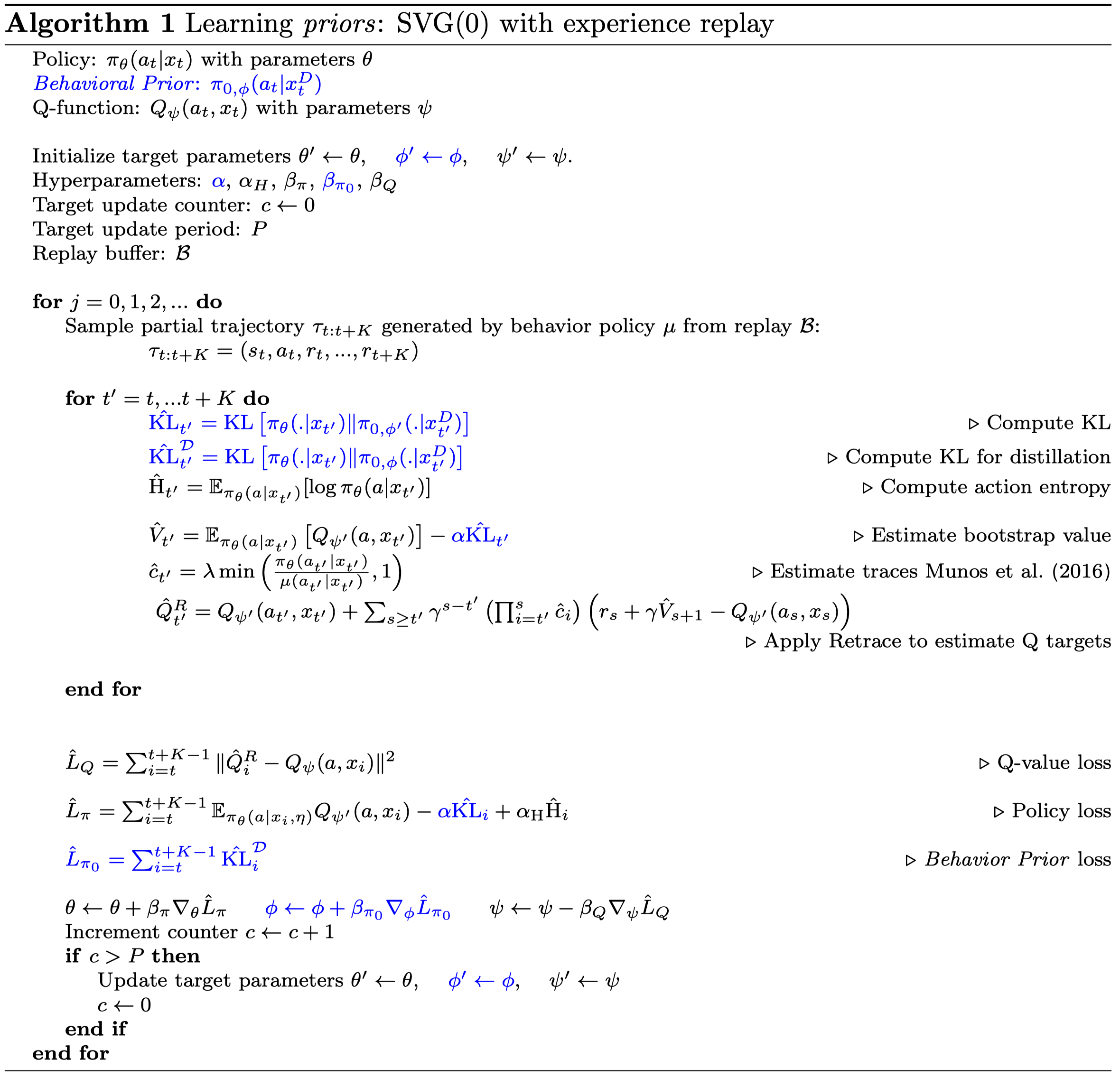
Notice that the \(Q\)-function is updated according to the retrace(\(\lambda\)) algorithm and we use the KL divergence against target prior \(\pi_{0,\phi’}\) in the actor and critic losses to provide stable learning signals. Also, it might be a good idea to use \(\pi_{\theta’}\) when computing the target Q value.
Structured Behavior Prior Models
So far, we have only considered \(\pi_0\) to be uni-modal Gaussian distributions. However, this may fail when the desirable prior is multi-modal, the common case when learning priors from multiple tasks (cf. Equation \((7)\)). To meet these involved situations, we utilizes latent variable models, a technique wildly used in probabilistic model to increase capacity, introduce inductive biases and model complex distribution.
We consider directed latent variable models for both \(\pi_0\) and \(\pi\) of the following form
\[\begin{align} \pi_0(\tau)=\int\pi_0(\tau|z)\pi_0(z)dz\tag 9\\\ \pi(\tau)=\int\pi(\tau|z)\pi(z)dz\tag{10} \end{align}\]where the latents \(z\) can be time varying, continuous or discrete, and can exhibit further structure. Notice that we also consider policies \(\pi\) with latent variables, which admits multiple solutions to solving the tasks. Moreover, the KL term towards a suitable prior can create pressure to learn a distribution over solutions, and augmenting \(\pi\) may make it easier to model these distinct solutions. (Hausman et al., 2018)
Simplified Form
Unfortunately, it’s difficult to directly compute the KL divergence between two complex distributions outlined in Equations \((9)\) and \((10)\). Instead, if we divide \(\pi\) into higher level \(\pi^H(z_t\vert x_t)\) and lower level \(\pi^L(a_t\vert z_t,x_t)\) components, we can derive the following upper bound for the KL term
\[\begin{align} D_{KL}(\pi(a_t|x_t)\Vert\pi_0(a_t|x_t))\le D_{KL}&(\pi^H(z_t|x_t)\Vert\pi_0^H(z_t|x_t))\\\ &+\mathbb E_{\pi^H(z_t|x_t)}[D_{KL}(\pi^L(a_t|z_t,x_t)\Vert \pi_0^L(a_t|z_t,x_t))]\tag{11} \end{align}\]Proof:
\[\begin{align} D_{KL}(\pi(a_t|x_t)\Vert\pi_0(a_t|x_t))&\le D_{KL}(\pi(a_t|x_t)\Vert\pi_0(a_t|x_t)) +\mathbb E_{\pi(a_t|x_t)}[D_{KL}(\pi^H(z_t|a_t, x_t)\Vert \pi_0^H(z_t|a_t, x_t))]\\\ &=\mathbb E_{\pi(a_t|x_t)}\left[\log{\pi(a_t|x_t)\over \pi_0(a_t|x_t)}\right]+\mathbb E_{\pi(a_t|x_t)} \left[\mathbb E_{\pi^H(z_t|a_t,x_t)}\left[\log{\pi^H(z_t|a_t,x_t)\over \pi_0^H(z_t|a_t, x_t)}\right]\right]\\\ &=\mathbb E_{\pi(a_t,z_t|x_t)}\left[\log{\pi(a_t,z_t|x_t)\over \pi_0(a_t,z_t|x_t)}\right]\\\ &=\mathbb E_{\pi^H(z_t|x_t)}\left[\log{\pi^H(z_t|x_t)\over \pi_0^H(z_t|x_t)}\right]+\mathbb E_{\pi^H(z_t|x_t)} \left[\mathbb E_{\pi^L(a_t|z_t,x_t)}\left[\pi^L(a_t|z_t,x_t)\Vert \pi_0^L(a_t|z_t, x_t)\right]\right]\\\ &=D_{KL}(\pi^H(z_t|x_t)\Vert\pi_0^H(z_t|x_t))+\mathbb E_{\pi^H(z_t|x_t)}[D_{KL}(\pi^L(a_t|z_t,x_t)\Vert \pi_0^L(a_t|z_t,x_t))] \end{align}\]where we use \(\pi^H\) to denote a conditional probability of \(z\) and use \(\pi^L\) and \(\pi\) to denote conditional probabilities of \(a\).
Intuition: The constraint between the higher level policies in Equation \((11)\) has two effects: it regularizes the higher level action space making it easier to sample from; and it introduces an information bottleneck between the two levels. The higher level thus ‘pays’ a price for every bit it communicates to the lower level. This encourages the lower level to operate as independently as possible to solve the task. By introducing an information constraint on the lower level, we can force it to model a general set of skills that are modulated via the higher level action \(z\) in order to solve the task.
Partial parameter sharing: An advantage of hierarchical structure is that it enables several options for partial parameter sharing. For instance, sharing the lower level controllers between the agent and the default policy allows skills to be directly reused. This amounts to a hard constraint that forces the KL between the lower levels to zero and results in the following objective
\[\begin{align} \mathcal J=\sum_{t}\mathbb E_{ \pi}\left[\gamma^tr(s_t,a_t)-\gamma^tD_{KL}(\pi(z_t|x_t)\Vert \pi_0(z_t|x_t))\right]\tag{12} \end{align}\]If we don’t consider the concept of hierarchy, Equation \((12)\) simply lifts the KL regularization from the policy to a latent variable inside the neural network.
In most of experiments, Tirumala et al. 2020 use a lower level policy shared between the prior and policy and find this structured prior performs better than unstructured prior, especially on complex tasks. Furthermore, they find additional performance gain in a separate lower level prior.
Algorithm
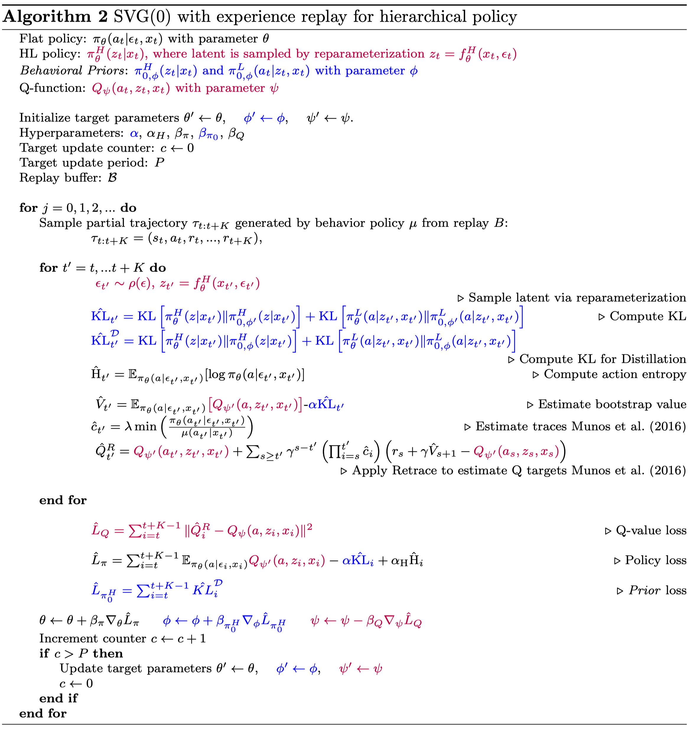
Several modifications are made compared to Algorithm 1
-
Besides policies, value functions are also conditioned on \(z\). This also changes the way of computing \(c_i\), which now becomes \(c_i=\lambda\min\left({\pi^H(z_i\vert x_i)\pi^L(a_i\vert x_i,z_i)\over \mu(a_i,x_i)},1\right)\). Notice that we consider the latent \(z\) when computing the current action probability but do not consider it in the behavior policy \(\mu\). This reduces the variance of the estimator.
-
When computing gradients to policy \(\pi\), we differentiate \(Q\) through action \(a\) but not through the latent \(z\), which empirically leads to better performance. This gives the following gradient
-
We add an additional entropy term to the policy loss to encourage exploration.
-
In practice, it may be desirable to sample \(z\) infrequently or hold it constant across multiple time steps to exhibit temporally consistent behavior. This gives us a similar structure as the one used in FTW.
References
>Tirumala, Dhruva, Alexandre Galashov, Hyeonwoo Noh, Leonard Hasenclever, Razvan Pascanu, Jonathan Schwarz, Guillaume Desjardins, et al. 2020. “Behavior Priors for Efficient Reinforcement Learning,” 1–58. http://arxiv.org/abs/2010.14274.
Vinyals, Oriol, Igor Babuschkin, Wojciech M. Czarnecki, Michaël Mathieu, Andrew Dudzik, Junyoung Chung, David H. Choi, et al. 2019. “Grandmaster Level in StarCraft II Using Multi-Agent Reinforcement Learning.” Nature 575 (November). https://doi.org/10.1038/s41586-019-1724-z.
Galashov, Alexandre, Siddhant M. Jayakumar, Leonard Hasenclever, Dhruva Tirumala, Jonathan Schwarz, Guillaume Desjardins, Wojciech M. Czarnecki, Yee Whye Teh, Razvan Pascanu, and Nicolas Heess. 2019. “Information Asymmetry in KL-Regularized RL.” ArXiv, 1–25.
Hausman, Karol, Jost Tobias Springenberg, Ziyu Wang, Nicolas Heess, and Martin Riedmiller. Learning an embedding space for transferable robot skills. In International Conference on Learning Representations, 2018.