
Introduction
In this post, we will discuss latent variable models used to model the marginal likelihood of the observed data, whose probabilistic distribution may be arbitrarily complex. A typical example we oftentimes see in machine learning is the Gaussian Mixture Model discussed in the previous post, in which we have
\[\begin{align} p(x)=\sum_z p(x|z)p(z) \end{align}\]where \( z \) indexes the Gaussian cluster, and \( p(x\vert z) \) is essentially a Gaussian distribution.
In reinforcement learning, we often see the conditional version of latent variable models, since the policy(i.e., the target of the conditional latent variable model) is expressed as the action distribution conditioned on a state.
One example is that used in multi-modal policies, in which we have
\[\begin{align} p(a|s)=\int p(a|s, z)p(z|s)dz \end{align}\]where \( p(z\vert s) \) may simply be a standard Gaussian distribution independent of \(s\), namely \( \mathcal N(0, 1) \), and \( p(a\vert s,z) \) is a Gaussian distribution represented by a network, which takes as inputs \( s \) and \( z \), and outputs \( a \). Because, for each \( z \), we have a corresponding Gaussian distribution \( p(a\vert s,z) \), integrating over \( z \), the model is able to model a multi-modal action distribution.
Variational Inference
First recall that our objective is to maximize the log likelihood \( \log p(x^{(i)}) \). Applying the latent variable model, we get
\[\begin{align} \log p(x^{(i)})=\log \int p(x^{(i)}, z)dz\tag {3} \end{align}\]The integral is the hard point that we want to get rid of since it makes Eq\( (3) \) intractable. One way to do that is to replace it with expectation. That is,
\[\begin{align} \log p(x^{(i)})&=\log\int p(x^{(i)}, z)dz\\\ &=\log\int p(x^{(i)}, z){q_i(z)\over q_i(z)}dz\\\ &=\log \mathbb E_{z\sim q_i(z)}\left[p(x^{(i)},z)\over q_i(z)\right]\\\ &\ge\mathbb E_{z\sim q_i(z)}\left[\log{p(x^{(i)},z)\over q_i(z)}\right]\\\ &=\mathbb E_{z\sim q_i(z)}\left[\log p(x^{(i)},z)\right]+\mathcal H(q_i)\tag {4} \end{align}\]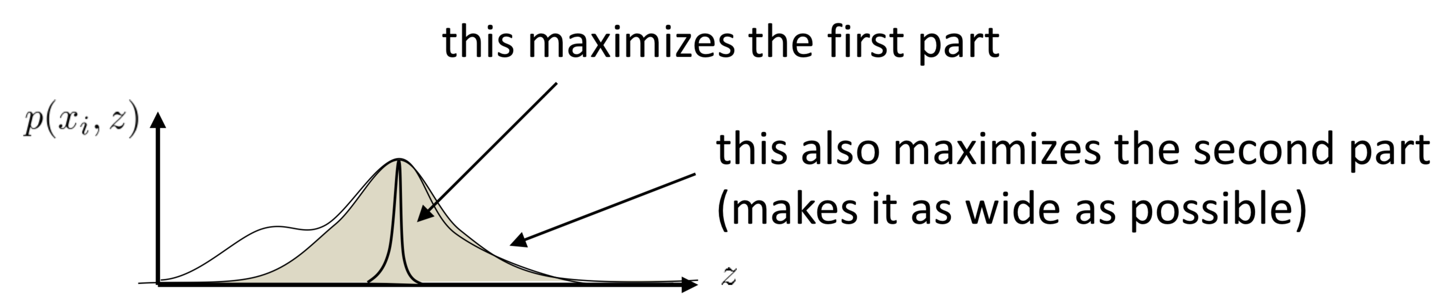
where the inequality is taken because of Jensen’s inequality and Eq.\( (4) \) is exactly the ELBO. These two terms have some nice intuitive interpretations: when we maximize the first term w.r.t. \( q_i \), we actually make \( q_i \) put more weights on the modes of \( p(x^{(i)}, z) \); on the other hand, maximizing the entropy of \( q_i \) spreads the distribution out, minimizing the amount of prior information built into the distribution. Together, \( q_i \) will tend to be like multiple Gaussians(since Gaussian distributions have the maximum entropy with a specified mean and variance) centered at the modes of \( p(x^{(i)},z) \). An illustration is given to the right.
Amortized Variational Inference
In Eq.\( (4) \) we have one \( q_i(z) \) for each data point \( x^{(i)} \), which is infeasible when dataset is large. To address this issue, we take \( q \) as a function of \( x \), outputting a distribution of \( z \) for each \( x^{(i)} \) (which is called amortized variational inference). Now we have
\[\begin{align} \log p_\theta(x^{(i)})=\mathbb E_{z\sim q_\phi(z|x^{(i)})}\left[\log p_\theta(x^{(i)}, z)\right]+\mathcal H(q_\phi)\tag {5} \end{align}\]The entropy term oftentimes could be analytically written down, and therefore it is easy to differentiate. Especially, for a Gaussian distribution, we have
\[\begin{align}\mathcal H(q_\phi)&=-\mathbb E\left[\log {1\over \sqrt{|2\pi\Sigma|}}e^{-{(x-\mu)^2\over 2\Sigma}}\right]\\\ &={1\over 2}\log |2\pi\Sigma| e\tag {6} \end{align}\]The first term in Eq.\( (5) \) can in fact be solved by the score function estimator, in which we have
\[\begin{align} \nabla_\phi\mathbb E_{z\sim q_\phi(z|x^{(i)})}\left[\log p_\theta(x^{(i)}, z)\right]=\mathbb E_{z\sim q_\phi(z|x^{(i)})}\left[\log p_\theta(x^{(i)}, z)\nabla_\phi \log q_\phi(z|x^{(i)})\right]\tag {7} \end{align}\]Eq.\( (7) \) generally has high variance since \( \log p_\theta(x^{(i)},z) \) is not restricted. Although one could use some variance reduction techniques, such as baseline, to mitigate such an issue, we can actually do better via the reparameterization trick as we did in the previous post. Specifically, for the case where \( q_\phi \) is a Gaussian distribution, we could compute \( z \) as
\[\begin{align} z=\mu_\phi(x)+\epsilon\sigma_\phi(x) \end{align}\]where \( \epsilon=\mathcal N(0, 1) \) is independent of \( \phi \). Eq.\( (7) \) now could be written as
\[\begin{align} \nabla_\phi\mathbb E_{z\sim q_\phi(z|x^{(i)})}\left[\log p_\theta(x^{(i)}, z)\right]=\mathbb E_{\epsilon\sim\mathcal N(0,1)}\left[\nabla_{\phi}\log p_\theta(x^{(i)}, \mu_\phi(x^{(i)})+\epsilon \sigma_\phi(x^{(i)}))\right]\tag {8} \end{align}\]Eq.\( (8) \) in general has lower variance than Eq.\( (7) \) because \( \log p_\theta(x^{(i)}, z) \), coming from sample, is more random than \( \epsilon \), whose variance is fixed to be \( 1 \). On the other hand, the reparameterization trick requires the latent variable \( p_\theta(x, z) \) to be continuous so that the log probability could be differentiable, while the score function estimator only requires \( q_\phi(z\vert x^{(i)}) \) to be differentiable. All in all, Eq.\( (8) \) should be preferred whenever possible.
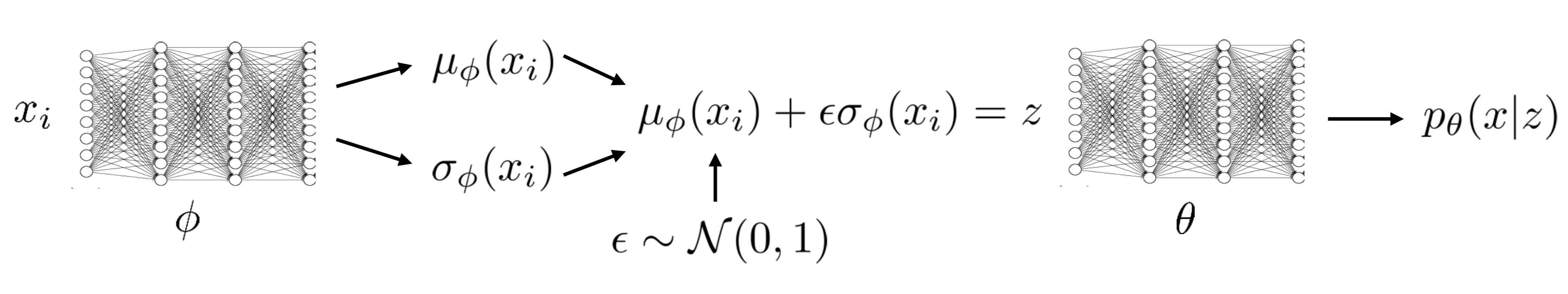
As a closure, the following figure illustrates the architecture of the above model
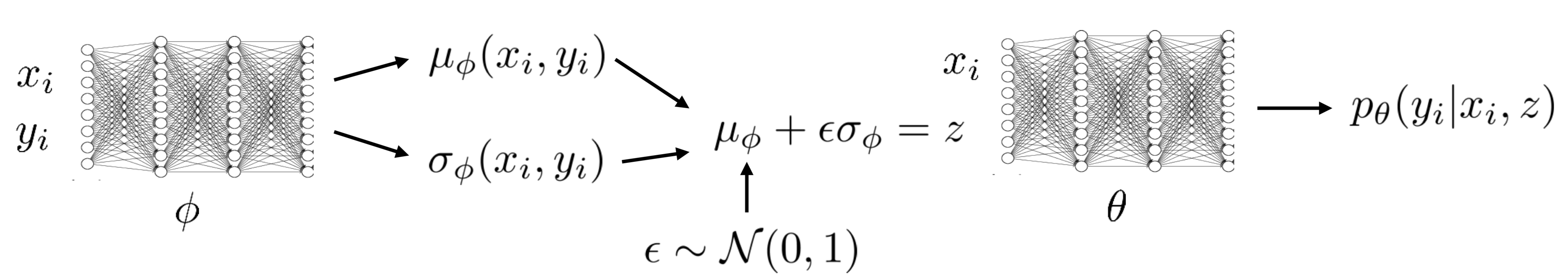
The same process can actually work with conditional models, where we have the ELBO
\[\begin{align} \mathcal L^{(i)}&=\mathbb E_{z\sim q_\phi(z|x^{(i)}, y^{(i)})}[\log p_\theta(y^{(i)}|x^{(i)},z)+\log p(z)]+\mathcal H(q_\phi(z|x^{(i)}, y^{(i)}))\tag {9}\\\ \mathrm{or}\quad\mathcal L^{(i)}&=\mathbb E_{z\sim q_\phi(z|x^{(i)}, y^{(i)})}[\log p_\theta(y^{(i)}|x^{(i)},z)+\log p(z|x^{(i)})]+\mathcal H(q_\phi(z|x^{(i)}, y^{(i)}))\tag{10} \end{align}\]Both Eq.\( (9) \) and Eq.\( (10) \) are feasible choices. The difference is that one’s latent variables depend on the prior \( x^{(i)} \) and the other’s don’t. The architecture of the conditional latent variable model is shown in the following figure.
References
CS 294-112 at UC Berkeley. Deep Reinforcement Learning Lecture 14