
Introduction
Gradient-based learning algorithms have been wildly used in deep learning and deep reinforcement learning in combination with neural networks. Its expressive power allows researchers to search in the space of architectures and objectives/losses that are both highly expressive and conducive to optimization.
In this post, we will first analyze two basic gradient estimators, and then walk through the formalism of stochastic computation graphs that help us compute gradient estimators.
Table of Contents
Basic Gradient Estimators
Suppose that \( x \) is a random variable, \( f \) is a function, and we are interested in computing the gradient estimator \( \nabla_\theta E_x[f(x)] \). There are two basic gradient estimators depending on how \( x \) is parameterized in terms of \( \theta \):
- \( x \) is sampled from a parameterized probability distribution, i.e., \( \mathbb E_{x\sim p(\cdot;\theta)}[f(x)] \). In this case, we generally end up with the score function (SF) estimator
since
\[\begin{align} \nabla_\theta \mathbb E_{x\sim p(\cdot;\theta)}[f(x)]&=\nabla_\theta\int f(x)p(x;\theta)dx\\\ &=\int f(x)\nabla_\theta p(x;\theta)dx\\\ &=\int f(x){\nabla_\theta p(x;\theta)\over p(x;\theta)}p(x;\theta)dx\\\ &=\int f(x)\nabla_\theta \log p(x;\theta)p(x;\theta)dx\\\ &=\mathbb E_{x\sim p(\cdot;\theta)}[f(x)\nabla_\theta\log p(x;\theta)] \end{align}\]This is valid iff \( p(x;\theta) \) is a continuous function of \( \theta \); however, it does not need \( f(x) \) to be a continuous function of \( x \) as we do not compute the derivative of \( f(x) \). An example is policy gradient methods, where we have the gradient estimator \( \mathbb E[\hat A(s,a)\nabla_\theta\log\pi_\theta(a\vert s)] \)
- \( x \) is a determinisitic, differentiable function of \( \theta \) and another random variable \( z \), i.e., \( \mathbb E_z[f(x(z,\theta))] \). Then we can use the pathwise derivative (PD) estimator, defined as follows
This is valid iff \( f(x(z,\theta)) \) is a continuous function of \( \theta \) for all \( z \). It is a well known pattern in deep neural networks, where \( z \) and \( x \) are the input and deterministic output of a neural network, respectively, and \( f \) is some continuous loss function, such as cross-entropy loss or mean square error. Also we could regard the PD estimator as the reparameterized function of the SF estimator. In particular, if \(p(x;\theta)\) is a Gaussian distribution, then in the PD estimator, we have
\[\begin{align} x(z,\theta)&=\mu+\sigma z\\\ \theta&=(\mu,\sigma)\\\ z&\sim\mathcal N(0, 1) \end{align}\]Stochastic Computation Graphs
Notations and Their Attributes
A stochastic computation graph is a directed, acyclic graph (DAG) with three types of nodes
- Input nodes, which represent inputs and parameters
- Deterministic nodes, which are functions of their parents. The gradients of deterministic nodes are computed according to the PD estimator as Eq. \( (2) \) suggests.
- Stochastic nodes, which are distributed conditionally on their parents. The gradients of stochastic nodes are computed according to the SF estimator as Eq. \( (1) \) suggests.
Each parent \( v \) of a non-input node \( w \) is connected to it by a directed edge \( (v, w) \). We say \( v \) influences \( w \) if there is a path from \( v \) to \( w \). Furthermore, if all intermediate nodes between \( v \) and \( w \) are deterministic, regardless of what type of node \( w \) is, we say \( v \) deterministically influences \( w \).
Deterministic influence has a nice property that gradients can be back-propagated through as long as all nodes along the path are differentiable. This does not hold if there is any stochastic node in the path since values of stochastic nodes are sampled from a probability distribution conditioned on their parents. Moreover, when there is a stochastic node in the path from \( v \) to \( w \), to compute the gradients with respect to \( v \), \( w \) does not even need to be differentiable.
Simple Examples
The following figure illustrates some simple examples
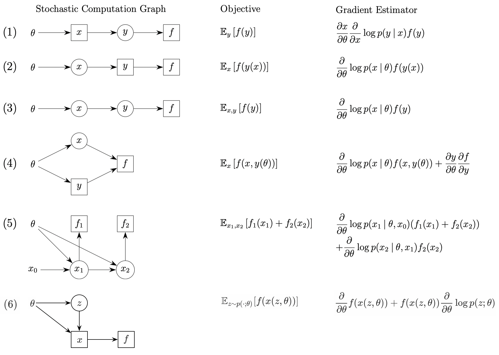
Here we only prove \( 5 \) and \( 6 \), others should be as clear as they are.
For \( 5 \), we have
\[\begin{align} \nabla_\theta\mathbb E_{x_1, x_2}[f_1(x_1)+f_x(x_2)]&= \nabla_\theta\left(\int \left(f_1(x_1)+\int f_2(x_2)p(x_2|x_1, \theta)dx_2\right )p(x_1|x_0,\theta)dx_1\right)\\\ &=\int \left(f_1(x_1)+\int f_2(x_2)p(x_2|x_1, \theta)dx_2\right)\nabla_\theta p(x_1|x_0,\theta)dx_1\\\ &\quad +\int \int \bigl( f_2(x_2)\nabla_\theta p(x_2|x_1,\theta)dx_2\bigr)p(x_1|x_0,\theta)dx_1\\\ &=\mathbb E_{x_1, x_2}\left[\left(f_1(x_1)+f_2(x_2)\right)\nabla_\theta\log p(x_1|x_0,\theta)+f_2(x_2)\nabla_\theta\log p(x_2|x_1,\theta)\right] \end{align}\]For \( 6 \), we have
\[\begin{align} \nabla_\theta\mathbb E_{z\sim p(\cdot;\theta)}[f(x(z, \theta))]&=\nabla_\theta\int f(x(z,\theta))p(z;\theta)dx\\\ &=\int \bigl(\nabla_\theta f(x(z, \theta))\bigr)p(z;\theta)+f(x(z, \theta))\nabla_\theta p(z;\theta)dx\\\ &=\int \bigl(\nabla_\theta f(x(z,\theta))+f(x(z, \theta))\nabla_\theta\log p(z;\theta)\bigr)p(z;\theta)dx\\\ &=\mathbb E_{z\sim p(\cdot;\theta)}\left[\nabla_\theta f(x(z,\theta))+f(x(z,\theta))\nabla_\theta\log p(z;\theta)\right] \end{align}\]Algorithm for Computing Gradient Estimator for Stochastic Computation Graph
Before dicussing the concrete algorithm, we first designate a set of cost nodes, which are scalar-valued and deterministic (Note that there is no loss of generality in assuming that the costs are deterministic — if a cost is stochastic, we can simply append a deterministic node that applies the identity function to it).
Now let’s take a look at the algorithm
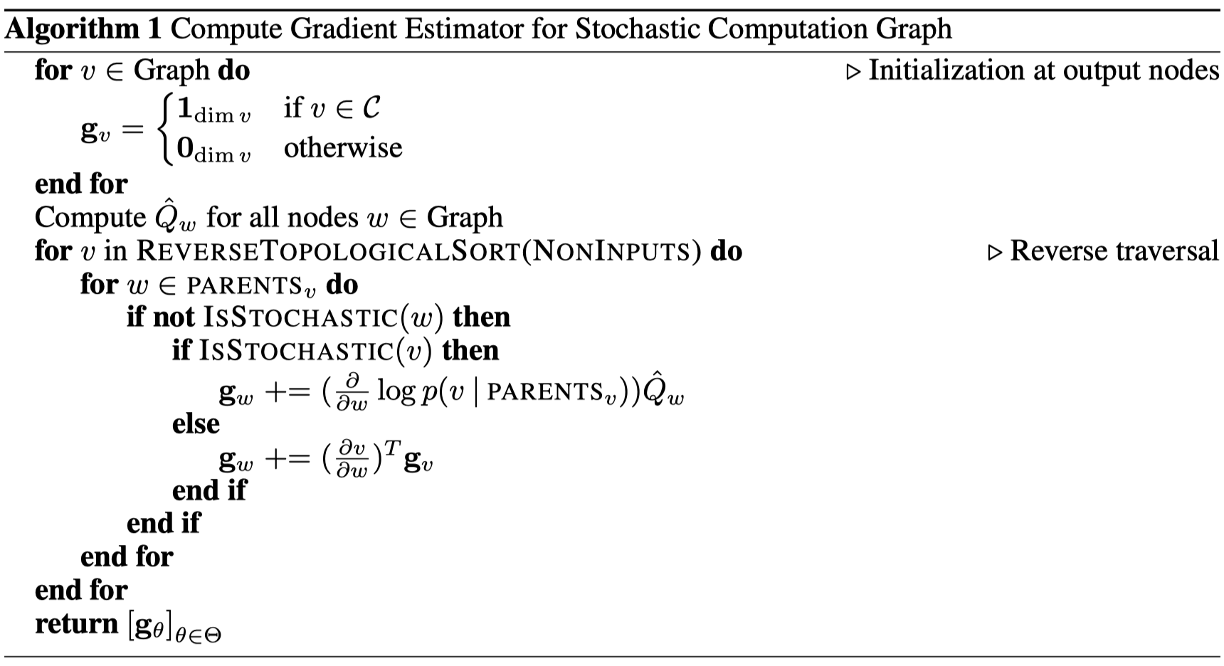
The algorithm is divided into three steps:
- Initialize the gradient of nodes in the graph with \( \mathbf 1 \) for cost nodes(since cost nodes are where the gradient computation starts from) and \( \mathbf 0 \) for the others.
- For each node \( w \) in the graph, calculate its downstream costs \( \hat Q_w \), sum of cost nodes influenced by that node.
- Compute the gradient estimator in reverse topological order. More concretely, we compute the gradient \( {\partial\over \partial w}\mathbb E\left[\sum_{c\in C}c\right] \) at each deterministic nodeand input node \( w \) as follows (stochastic nodes are omitted since their gradients will not get back-propagated): For edge \( (w, v) \), if \( v \) is deterministic, we compute the PD estimator \( (2) \) w.r.t. \( w \), otherwise we compute the SF estimator \( (1) \). In the end, we add up all the gradient estimates w.r.t. \( w \) to obtain \( {\partial\over \partial w}\mathbb E\left[\sum_{c\in C}c\right] \).
References
John Schulman et al. Gradient Estimation Using Stochastic Computation Graphs