
Introduction
In July 2020, Liu et al. introduced a set of unified normalization-activation layers, namely EvoNorm found by AutoML. In this post, we present EvoNorm as well as the evolution process of finding them, which is rather intersting.
This post is organized as follows:
- First, we present the result EvoNorm.
- Then we starts from the search space and see a naive random search method is ineffective due to the large spase search space and can easily fail to generalize across architecture.
- At last, we discuss the evolution method proposed by Liu et al.
EvoNorm
Two normalization-activation layers are found to be most effective across experiments:
- The batch-dependent layer EvoNorm-B0:
where \(\sqrt{s_{b,w,h}(x)}\) is the standard deviation computed along the batch and spatial dimensions of \(x\) and \(\sqrt{s_{w,h}}\) is the standard deviation computed along the spatial dimensions of \(x\). \(\gamma\) and \(\beta\) are the scale and bias in a normal linear layer.
- The batch-independent layer EvoNorm-S0:
where \(\sigma\) is the sigmoid function.
Interestingly, Both of them normalize data using the standard deviation but neither centralizes the data.
Search Space
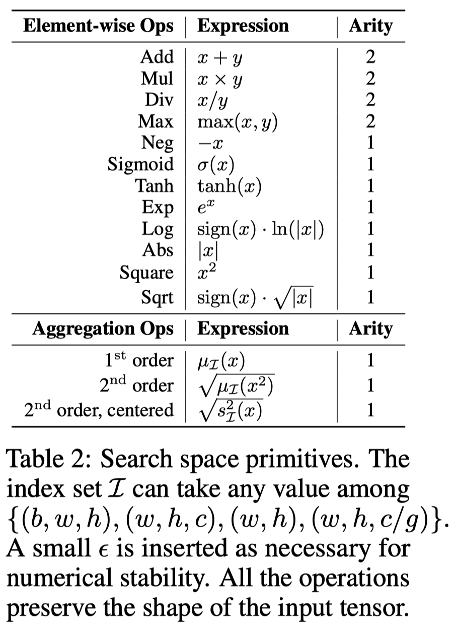
**Layer representation: **We represent each normalization-activation layer as a computation graph that transform an input tensor to an output tensor. The computation graph has \(4\) initial nodes, including the input tensor and three auxiliary nodes: a constant zero tensor, and two trainable vectors \(v_0\) and \(v_1\) along the channel dimension initialized as \(0\)’s and \(1\)’s, respectively. We restrict the total number of nodes in the graph to \(4+10=14\). Each intermediate nodes in the graph represents the outcome of either a unary or binary operations (shown in Table 2), where \(x_\mathcal I\) represents a subset of \(x\)’s elements along the dimensions indicated by \(\mathcal I\).
Random Graph Generation: A random computation graph can be generated sequentially from the initial nodes using the operations from Table 2. In their early experiments, they took \(5000\) random samples from the search space and plugged them into three architectures on CIFAR-10. Unfortunately, none of them outperforms BN-ReLU, indicating the high sparsity of the search space. Another observation is that randomly generated layers often suffer from the generalization issue across architectures – some layers performs well on one architecture can fail completely on the others.
Search Method
Evolution
The new method is an evolution algorithm based on a variant of tournament selection. At each step, a tournament is formed based on a random subset(\(5\%\)) of the population. The winner of the tournament is allowed to produce offspring, which will be evaluated and added into the population. The population, thus, improves as the process repeats. We also regularize the evolution by maintaining only a fixed number of the most recent portion of the population. An offspring is produced in three steps. First, we select a intermediate node uniformly at random. Then we replace its current operation with a new one in Table 2 uniformly at random. Finally, we select new predecessors for this node among existing nodes in the graph uniformly at random. In this way, the newly replaced-in node is connected to the same successor as the original node but may to a different predecessor(s).
Rejection protocols to address high sparsity of the search space
Although evolution improves sample efficiency over random search, it does not resolve the high sparsity issue of search space. Liu et al. propose two rejection protocols to filter out bad layers after short training. A layer must pass both tests to be added to the population
- Quality. We discard layers that achieves less than \(20\%\) CIFAR-10 validation accuracy after training for \(100\) steps. As the vast majority of the candidate layers establish poor accuracy, this mechanism ensures compute resources to concentrate on the full training of a small number of promising candidates. Empirically, this speeds up the search by up to two orders of magnitude.
- Stability. We also reject layers subject to numerical instability. The basic idea is to stress-test the candidate layer by adversarially adjusting the model weights \(\theta\) towards the direction of maximizing the network’s gradient norm. This helps reveal the potential exploding gradient problems of the network. Formally, let \(\ell(\theta,G)\) be the traning loss of a model when paired with computation graph \(G\) computed based on a small batch of images. Instability of training is reflected by the worst-case gradient norm: \(\max_\theta\Vert\partial\ell(\theta, G)\partial\theta\Vert_2\). We seek to maximize this value by perform gradient ascent along the direction of \(\partial\Vert\partial\ell(\theta, G)\partial\theta\Vert_2\over \partial\theta\) up to \(100\) steps. Layers whose gradient norm exceeding \(10^8\) are rejected. The stability test focuses on robustness because it considers the worst case, hence is complementary to the quality test. This test is highly efficient-gradients as many layers are forced to quickly blow up in less than 5 steps
Multi-architecture evaluation to promote strong generalization
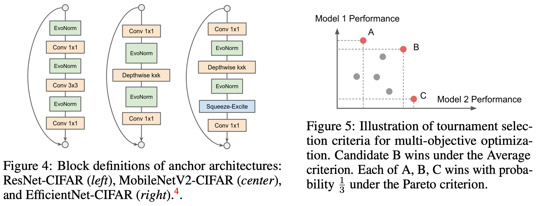
To promote strong generalization, Liu et al. formulate the search as a multi-objective optimization problem, where each candidate layer is always evaluated over multiple different anchor architectures to obtain a set of fitness scores. The architectures chosen include ResNet50(v2), MobileNetV2 and EfficientNet-B0. Widths and strides are adapted w.r.t. the CIFAR-10 dataset. See Figure 4 for the basic block of these architectures.
Tournament Selection Criterion. As now each layer associates to multiple architecture, there are multiple ways to decide the tournament winner:
- Average: Layer with the highest average accuracy wins (e.g. B in Figure 5 wins)
- Pareto: A random layer on the Pareto frontier wins (e.g., A, B, C in Figure 5 are equal likely to win)
Empirically, Liu et al. observed that ResNet has a higher accuracy variance than the other two architectures. Hence, under the average criterion, the search will bias towards helping ResNet. They therefore propose to use the Pareto frontier criterion to avoid this bias.
References
Liu, Hanxiao, Andrew Brock, Karen Simonyan, and Quoc V. Le. 2020. “Evolving Normalization-Activation Layers,” 1–17. http://arxiv.org/abs/2004.02967.