
Introduction
We discuss MobileNet families, proposed by researchers in Google, that aims to reduce the computation and memory requirements of modern deep CNNs, while maintaining high performance.
Terminologies
**Depth: ** The number of blocks
**Width: ** The number of channels/filters
**Resolution: ** The feature map size \(H\times W\)
MobileNetV1
The core contribution of MobileNet is depthwise separable convolutions, which aims to reduce computation and memory requirements of modern deep CNNs. Depthwise separable convolutions factorize a standard convolution into a depthwise convolution and a \(1\times 1\) convolution called a pointwise convolution: The depthwise convolution filters each input channel and the pointwise convolution combines the outputs.
Considering a input tensor of shape \(H\times W\times C\), the depthwise convolution separably applies \(C\) $K\times K$ kernels to each input channel. This convolution preserves the shape of the tensor and has a computational cost of
\[\begin{align} \underbrace {H\cdot W\cdot C}_\text{total number of operations}\cdot \underbrace{K\cdot K}_\text{cost of each operation}\tag {1} \end{align}\]The pointwise convolution combines the filterred feature maps with a \(1\times 1\) convolution. This yields a \(H\times H\times C’\) tensor with a computation cost of
\[\begin{align} \underbrace{H\cdot W}_\text{total number of operations}\cdot \underbrace{C\cdot C'}_\text{cost of each operation}\tag {2} \end{align}\]Compare to standard convolution, which requires
\[\begin{align} \underbrace {H\cdot W}_\text{total number of operations}\cdot \underbrace{C\cdot C'\cdot K\cdot K}_\text{cost of each operation}\tag {3} \end{align}\]The reduction in computation is
\[\begin{align} &{H\cdot W\cdot C\cdot K\cdot K+H\cdot W\cdot C\cdot C'}\over{H\cdot W\cdot C\cdot C'\cdot K\cdot K}\\\ =&{1\over C'}+{1\over K^2}\tag {4} \end{align}\]When using \(3\times 3\) depthwise separable convolutions, it uses between \(8\) to \(9\) times less computation than standard convolutions at only a small reduction in accuracy.
Comparing Equations \((1)\) and \((2)\), we can see that depthwise separable convolution puts nearly all of the computation into dense \(1\times 1\) convolutions. However, contrasting to standard convolutions implemented by im2col followed by optimized general matrix multiply(GEMM), \(1\times 1\) convolutions does not require im2col for initial reordering and can be implemented directly with GEMM.
Despite the above theoretical arguments, I find the depthwise convolution is slower than standard convolution in practice (with float32, but someone said the performance gain will be spotted with float16). Gholami et al. explained:
The reason for this is the inefficiency of depthwise separable convolution in terms of hardware performance, which is due to its poor arithmetic intensity (ratio of compute to memory operations) [24]. This inefficiency becomes more pronounced as higher number of processors are used, since the problem becomes more bandwidth bound.
While the above explanation is a little obscure, Bello et al. 2021 provides a explanation easier to approach:
In custom hardware architectures (e.g. TPUs and GPUs), FLOPs are an especially poor proxy because operations are often bounded by memory access costs and have different levels of optimization on modern matrix multiplication units (Jouppi et al., 2017). The inverted bottlenecks used in EfficientNets employ depthwise convolutions with large activations and have a small compute to memory ratio (operational intensity) compared to the ResNet’s bottleneck blocks which employ dense convolutions on smaller activations. This makes EfficientNets less efficient on modern accelerators compared to ResNets.
In other words, depthwise convolutions are less compute efficient and require more memory access. Therefore, memory access(or bandwidth) become the bottleneck.
MobileNetV2
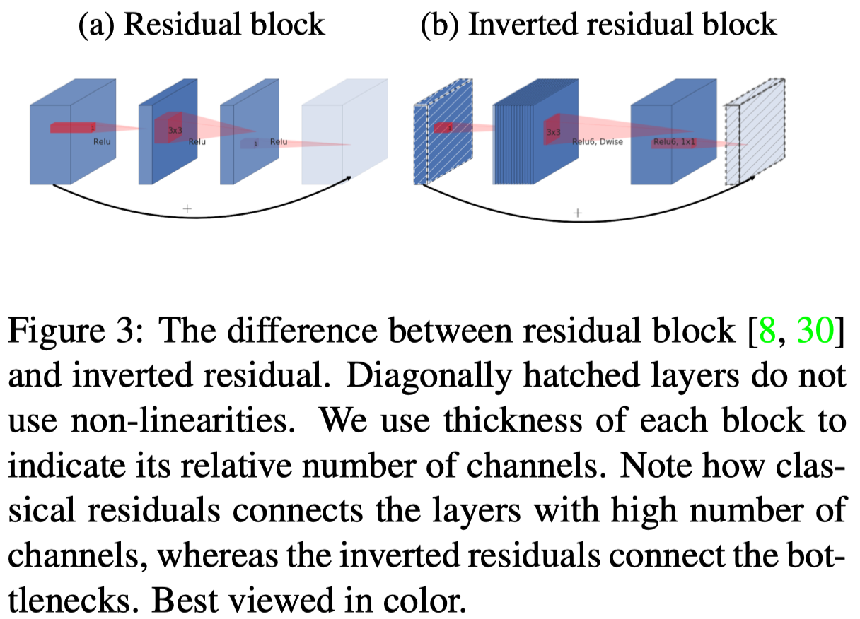
MobileNetV2 introduces a novel layer module: the inverted residual with linear bottleneck. Taking from the intuition that manifolds of interest in neural networks could be embedded in low-dimensional spaces, Sandler et al. propose inverted residual block that connects layers with low number of channels. See figure 3 for a comparison between residual block and its inverted version.
Notice that
- The inverted residual block also uses depthwise separable convolutions in the residual branch to separate filter and combine operations
- ReLUs in Figure 3.b is mislabelled. In practice, ReLU6 is used after the first two layers but not the last convolution because when the input to the residual block has the same capacity as the output, ReLU may cause a loss of information as it zeros-out negative values. (see the following intuition for more details)
Intuitively, in inverted residual block, we expect the input tensor with lower number of channels carries all the information needed for the following operations. However, filtering a lower dimensional tensor with ReLU activation may cause loss of information due to limited expressive power of a convolution and negative values being zeroed-out. Therefore, we expand it with a \(1\times 1\) convolution to make it more expressive for the following operations. Then we apply a depthwise separable convolution for memory efficiency. At last, we project the resulting feature maps back into the original size using a \(1\times 1\) convolution without any non-linearity. The non-linearity is used because we don’t want any loss of information, introduced by ReLU, between the input and output of the inverted residual block.
Also, EfficientNet(Tan&Le 2019) consists of mobile inverted bottleneck (MBConv).
MobileNetV3
MobileNetV3 use platform-aware network search and NetAdapt to search for the global network architectures and filters for each layers. Besides those search methods, Howard et al. redesign several computationally intensive layers and nonlinearities. We summarize them as follows
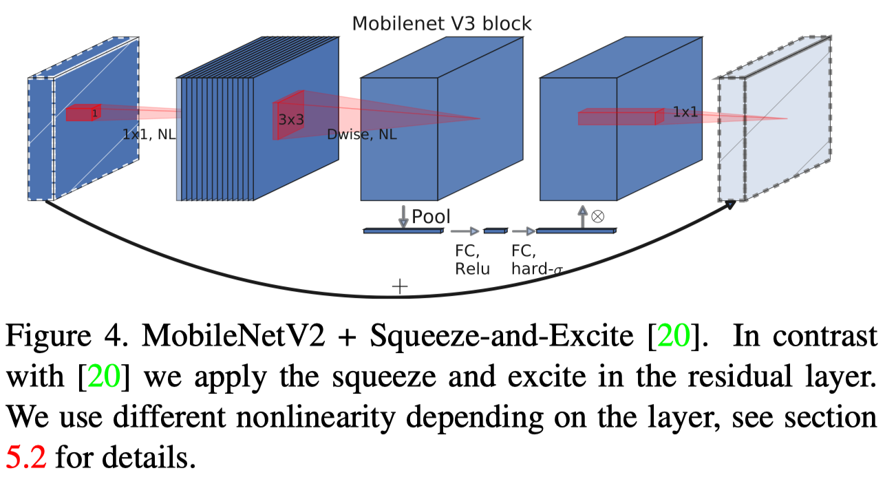
- SE block is appended after the depthwise convolutional layer with a reduction ratio of \(.25\). The output activation is replaced by the hard sigmoid to reduce computational cost as shown in figure 4
-
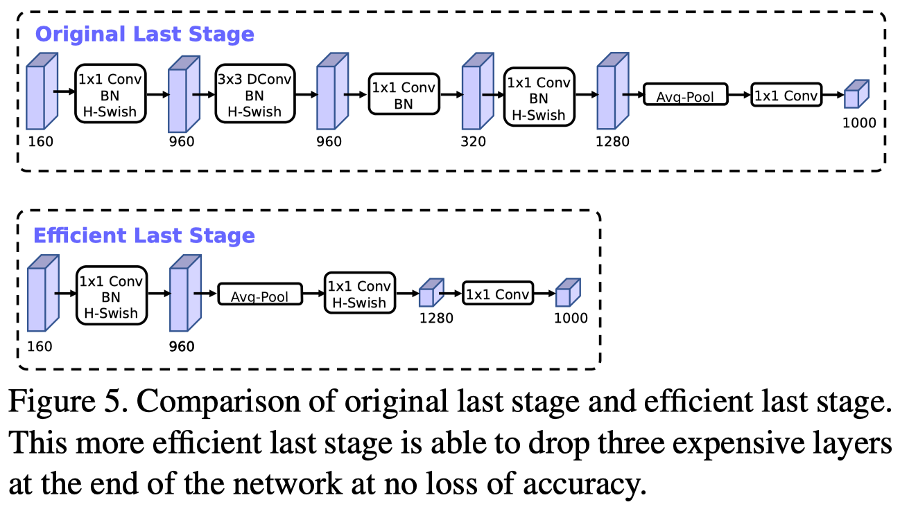
The last layer is redesigned as shown in Figure 5 to reduce the computational cost. This reduces the latency by \(7\) milliseconds and reduces the number of operations by \(30\) millions MAdds with almost no loss of accuracy.
-
swish activation is replaced by a hard version. The original swish is defined as \(\text{swish}(x)=x\sigma(x)\). As the sigmoid function is much more expensive to compute on mobile devices, Howard et al. introduce a hard version as \(\text{h-swish}(x)=x{\text{ReLU6}(x+3)\over 6}\). Howard et al. also find most of the benefits swish are realized by using them only in the deeper layers. Thus, they only use h-swish at the second half of the model.
References
Howard, Andrew G., Menglong Zhu, Bo Chen, Dmitry Kalenichenko, Weijun Wang, Tobias Weyand, Marco Andreetto, and Hartwig Adam. 2017. “MobileNets: Efficient Convolutional Neural Networks for Mobile Vision Applications.” http://arxiv.org/abs/1704.04861.
Sandler, Mark, Andrew Howard, Menglong Zhu, Andrey Zhmoginov, and Liang Chieh Chen. 2018. “MobileNetV2: Inverted Residuals and Linear Bottlenecks.” Proceedings of the IEEE Computer Society Conference on Computer Vision and Pattern Recognition, 4510–20. https://doi.org/10.1109/CVPR.2018.00474.
Howard, Andrew, Mark Sandler, Bo Chen, Weijun Wang, Liang Chieh Chen, Mingxing Tan, Grace Chu, et al. 2019. “Searching for MobileNetV3.” Proceedings of the IEEE International Conference on Computer Vision 2019-October: 1314–24. https://doi.org/10.1109/ICCV.2019.00140.