
Introduction
In the previous post, we discussed a specific neural network architecture for meta-learning named SNAIL, which utilizes temporal convolutions and attention to learn how to aggregate contextual information and distill useful information from that context. In this post, we will discuss an optimization algorithm, namely Model-Agnostic Meta-Learning(MAML), introduced by Finn et al. 2017. Unlike traditional optimization algorithms that train the model to optimize a specific task, this method trains the model to be easy to fine-tune. Besides its simplicity and effectiveness, a potential benefit of this approach is that it does not place any constraints on the model architecture, therefore, it can be readily combined with arbitrary networks. Furthermore, it can also be used with a variety of loss functions, which makes it applicable to a variety of different learning processes.
TL; DR
MAML learns a model that can be fast adapted to a new task within several gradient steps. This is achieved by directly minimizing the task loss for the adapted model. The following optimization problem shows an example for a single-step MAML
\[\begin{align} \min_\theta &\sum_{\mathcal T_i\sim p(\mathcal T)}\mathcal L_{\mathcal T_i}(f_{\theta'_i})\\\ where\quad \theta_i'=&\theta-\alpha\nabla_\theta\mathcal L_{\mathcal T_i}(f_\theta) \end{align}\]Model-Agnostic Meta-Learning
The idea behind MAML is simple: it optimizes for a set of parameters such that when a gradient step is taken w.r.t. a particular task \(i\), the parameters are close to the optimal parameters \(\theta_i\) for task \(i\). Therefore, the objective of this approach is to learn an internal feature that is broadly applicable to all tasks in a task distribution \(p(\mathcal T)\), rather than a single task. It achieves this by minimizing the total loss across tasks sampled from the task distribution \(p(\mathcal T)\).
\[\begin{align} \min_\theta &\sum_{\mathcal T_i\sim p(\mathcal T)}\mathcal L_{\mathcal T_i}(f_{\theta'_i})\tag 1\\\ where\quad \theta_i'=&\theta-\alpha\nabla_\theta\mathcal L_{\mathcal T_i}(f_\theta) \end{align}\]Note that we do not actually define an additional set of variables \(\theta_i’\) here. \(\theta’_i\) is just computed by taking several gradient steps from \(\theta\) w.r.t. task \(i\)—this step is generally called the inner loop learning, in contrast to the outer loop learning in which we optimize Eq.(1). If we take the inner loop learning as fine-tuning \(\theta\) with respect to task \(i\), then Eq.\((1)\) equally says that we optimize an objective in the expectation that the model does well on some task from the same task distribution after respective fine-tuning.
Another thing worth attention is that when we optimize Eq.\((1)\), we will eventually end up computing Hessian-vector products. The authors have conducted some experiments using a first-order approximation of MAML on supervised learning problems, where these second derivatives are omitted(which could be achieved programmatically by stopping computing the gradient of \(\nabla_\theta \mathcal L_{\mathcal T_i}(f_\theta)\)). Note that the resulting method still computes the meta-gradient at the post-update parameter values \(\theta_i’\), which provides for effective meta-learning. Experiments demonstrated that the performance of this method is nearly the same as that obtained with full second derivatives, suggesting that the most of the improvement in MAML comes from the gradients of the objective at the post-update parameter values, rather than the second order updates from differentiating through the gradient update.
Visualize MAML
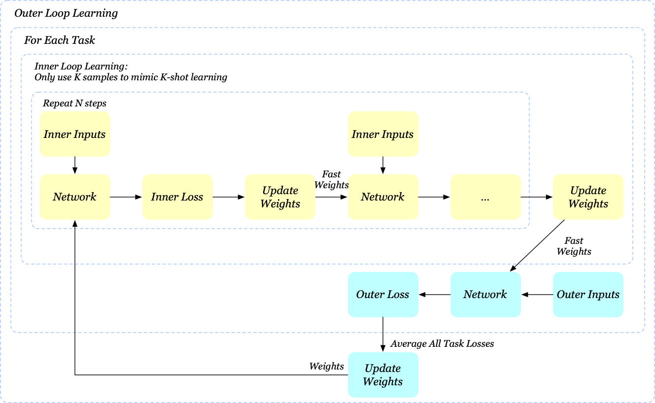
If the inner loop learning is repeated \(N\) times, MAML only uses the final weights for outer loop learning. As we will see in a future post, this could be troublesome, causing unstable learning when \(N\) is large.
Algorithm
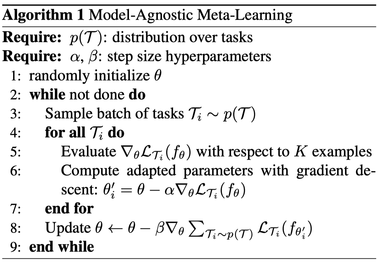
It now should be straightforward to see the algorithm
The reinforcement learning version is
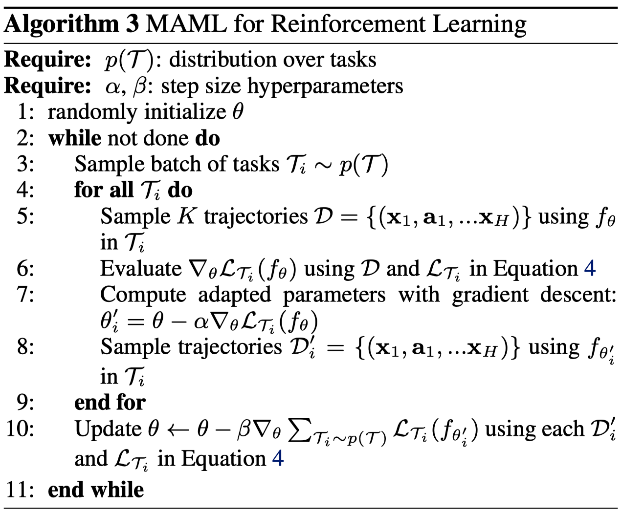
where steps 6 and 7 perform one general policy gradient step. Note that we resample trajectories after the network has been updated according to a specific task. This makes sense since \(\mathcal L_{\mathcal T_i}(f_{\theta_i’})\) should be evaluated under the new policy with parameters \(\theta_i’\).
Discussion
No Free Lunch
The generalization power of MAML actually comes with a price. Notice that MAML does not try to achieve a certain task goal. Instead, it is optimized so that it can perform well after a few gradient steps. As a result, in reinforcement learning, the policy it produces may not interact with the environment in a desirable way, which, in turns, influences the data distribution. Worse still, when cooperating with policy gradient methods, where the surrogate loss does not rightfully reflect what the agent is trying to achieve, MAML may be even more fragile.
Another noticeable thing is the computation cost. Even though we omit the second derivative, the computational and memory costs of MAML grow with the number of inner gradient steps and tasks we selected at each step.
References
- Chelsea Finn, Pieter Abbeel, Sergey Levine. Model-Agnostic Meta-Learning for Fast Adaptation of Deep Networks
- Tim Salimans et al. Weight Normalization: A Simple Reparameterization to Accelerate Training of Deep Neural Networks