Introduction
In the previous post, we discussed Model Agnostic Meta-Learning(MAML). We now address some issues raised in MAML and discuss potential solutions based on “How To Train Your MAML”, by Antreas et al. 2019.
Problems and Solutions
Training Instability
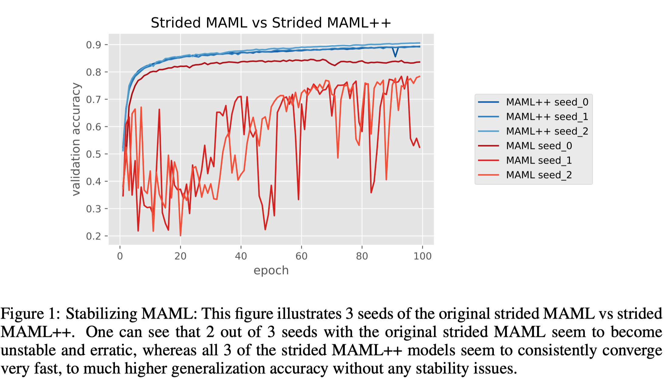
MAML training could be unstable depending on the neural network architecture and overall hyperparameter setup. For example, Antreas et al. 2019 found that simply replacing maxpooling layers with strided convolutional layers rendered it unstable as Figure 1 suggests. They conjectured the instability was caused by gradient degradation(either gradient explosion or vanishing gradient), which in turns caused by a deep network. To see this, we review the visualized MAML process illustrated in the previous post
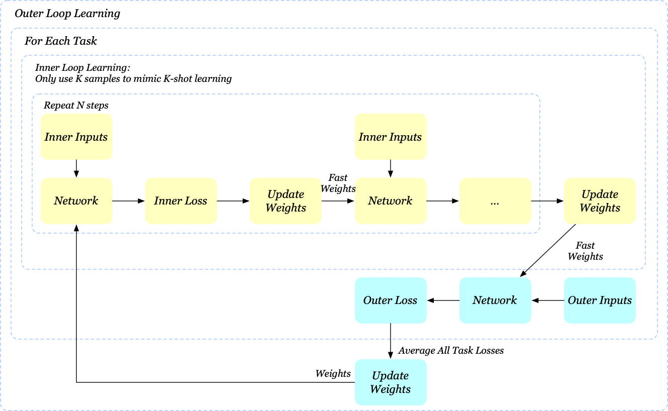
Assuming the network is a standard 4-layer convolutional network followed by a single linear layer, if we repeat the inner loop learning \(N\) times, then the inference graph is comprised of \(5N\) layers in total, without any skip-connections. Since the original MAML only uses the final weights for the outer loop learning, backpropagation has to pass through all \(5N\) layers, which makes sense of the gradient degradation.
We could adopt a similar idea from GoogLeNet to ease the gradient degradation problem by computing the outer loss after every inner step. Specifically, we now have the outer loop update
\[\begin{align} \theta = \theta-\beta\nabla_\theta\sum_{i=1}^B\sum_{j=1}^Nw_j\mathcal L_{T_i}(f_{\theta_j^i}) \end{align}\]where \(\beta\) is a learning rate, \(\mathcal L_{T_i}(f_{\theta_j^i})\) denotes the outer loss of task \(i\) when using the base-network weights after \(j\)-inner-step update and \(w_j\) denotes the importance weight of the outer loss at step \(j\). We also visualize this process for better comparison
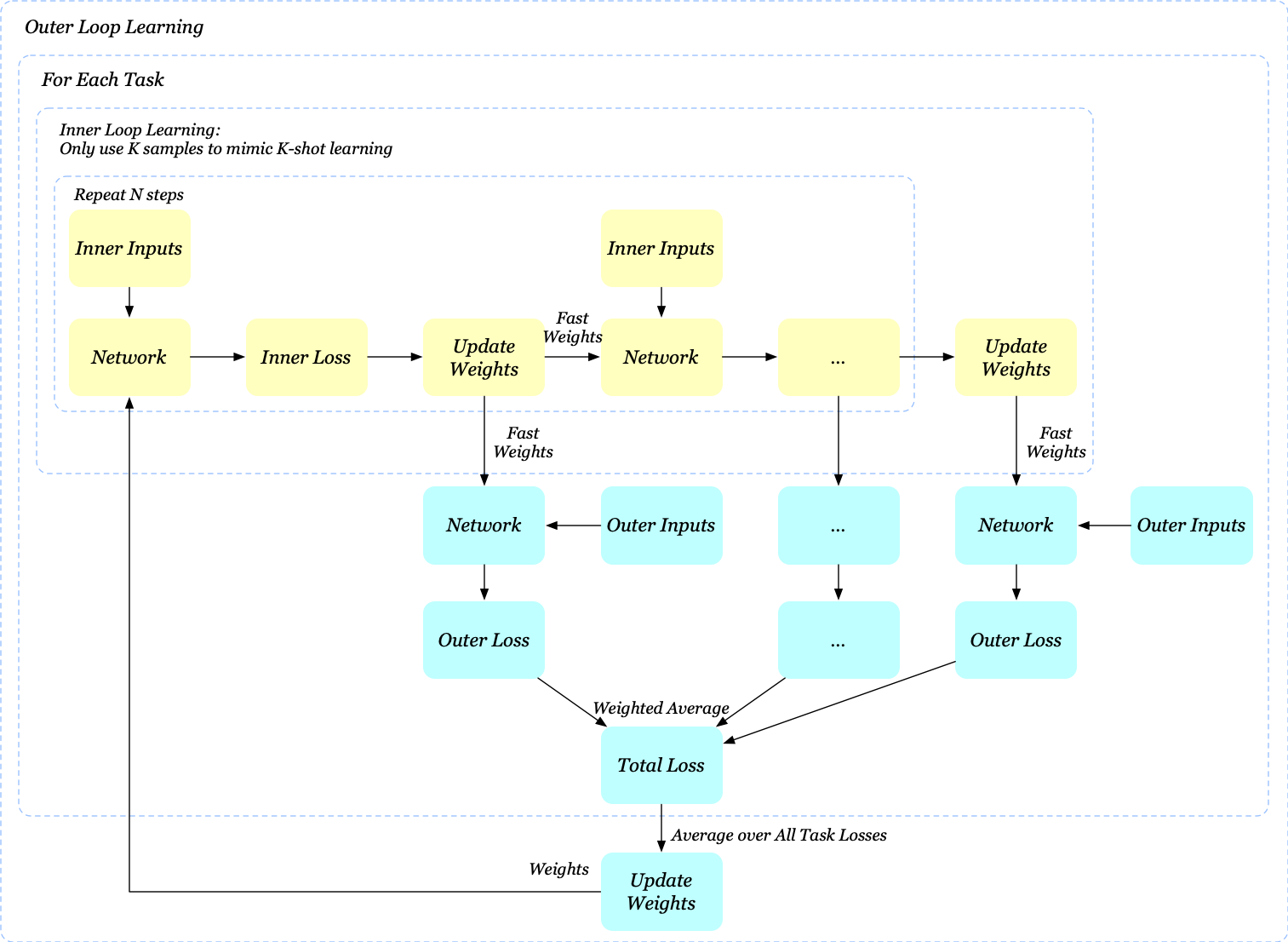
In practice, we initialize all losses with equal contributions towards the loss, but as iterations increase, we decrease the contributions from earlier steps and slowly increase the contribution of later steps. This is done to ensure that as training progresses the final step loss receives more attention from the optimizer thus ensuring it reaches the lowest possible loss. If the annealing is not used, the final loss might be higher than with the original formulation.
Second Order Derivative Cost
MAML reduces the second order derivative cost by completely ignoring it. This could impair the final generalization performance in some cases.
Solution: Derivative-Order Annealing (DA)
The authors of MAML++ propose to use the first-order gradient for the first 50 epochs of the training phase, and to then switch to second-order gradients for the remainder of the training phase. An interesting observation is that this derivative-order annealing showed no incidents of exploding or diminishing gradients, contrary to second-order only MAML which were more unstable. Using first-order before starting to use second-order derivatives can be used as a strong pretraining method that learns parameters less likely to produce gradient explosion/diminishment issues.
Absence of Batch Normalization Statistic Accumulation
MAML does not use running statistics in batch normalization. Instead, the statistics of the current batch is used. This results in batch normalization being less effective since the parameters learned have to accommodate for a variety of different means and standard deviations from different tasks.
Solution: Per-Step Batch Normalization Running Statistics, Per-Step Batch Normalization Weights and Biases (BNRS + BNWB)
A naive implementation of batch normalization in the context of MAML would accumulate running batch statistics across all update steps of the inner-loop learning. Unfortunately, this would cause optimization issues and potentially slow down or altogether halt optimization. This issue stems from a wrongly placed assumption: when we maintained the running statistics shared across all inner loop updates of the network, we assumed the initial model and all its updated iterations had similar feature distributions. Obviously, this assumption is far from correct. A better alternative is to store per-step running statistics and learn per-step batch normalization parameters for each of the inner-loop iterations.
Shared Inner Loop Learning Rate
One issue that affects the generalization and convergence speed is the issue of using a shared learning rate for all parameters and all update-steps. Having a fixed learning rate requires doing multiple hyperparameter searches to find the correct learning rate for a specific dataset, which can be computationally costly, depending on how search is done. Moreover, while gradient is an effective direction for data fitting, a fixed learning rate may easily lead to overfitting under the few-shot regime.
Solution: Learning Per-Layer Per-Step Learning Rates (LSLR)
To avoid potential overfitting, one approach is to determine all learning factors in a way that maximizes generalization power rather than data fitting. Li et al.[2] propose to learn a learning rate for each parameter in the base-network. The inner loop update now becomes \(\theta’=\theta-\alpha\circ\nabla_\theta\mathcal L_{T_i}(f_{\theta})\), where \(\alpha\) is a vector of learnable parameters with the same size as \(\theta\), and \(\circ\) denotes element-wise product. The resulting method, namely Meta-SGD, has been demonstrated to achieve a better generalization performance than MAML, with the cost of increasing learning parameters and computational overhead. Note that we do not put the constraint of positivity on the learning rate. Therefore, we should not expect the inner-update direction follows the gradient direction.
Considering the induced cost of Meta-SGD, Antoniou et al. propose learning a learning rate for each layer in the network as well as learning different learning rate for each adaptation of the base-network as it takes steps. For example, assuming the base-network has L layers and the inner loop learning consists of N steps updates, we now introduce \(LN\) additional learnable parameters for the inner loop learning rate.
Fixed Outer Loop Learning Rate
MAML uses Adam with a fixed learning rate to optimize the meta-objective. It has been shown in some literature that an annealing learning rate is crucial for generalization performance. Furthermore, having a fixed learning rate might mean that one has to spend more time tuning the learning rate.
Solution: Cosine Annealing of Meta-Optimizer Learning Rate(CA)
Antoniou et al. propose applying the cosine annealing scheduling(Loshchilov & Hutter[3]) on the meta-optimizer. The cosine annealing scheduling is defined as
\[\begin{align} \beta=\beta_{min}+{1\over 2}(\beta_{max}-\beta_{min})\left(1+\cos\left({T\over T_{max}}\pi\right)\right) \end{align}\]where \(\beta_{min}\) denotes the minimum learning rate, \(\beta_{max}\) denotes the initial learning rate, \(T\) is the number of current iterations, \(T_{max}\) is the maximum number of iterations. When \(T=0\), learning rate \(\beta=\beta_{max}\). Once \(T=T_{max}\), \(\beta=\beta_{min}\). In practice, we might want to bound \(T\) to be \(T_{max}\) to avoid restart.
Experimental Results
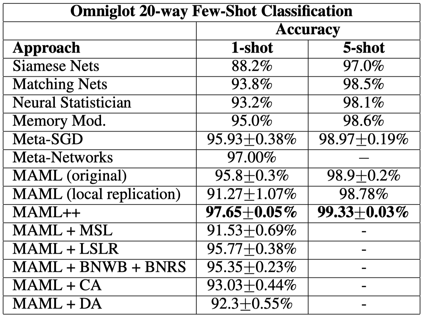
Finally,As show we present some Experimental results for completeness.
First we show individual improvement on the MAML in the 20-way Omniglot tasks.
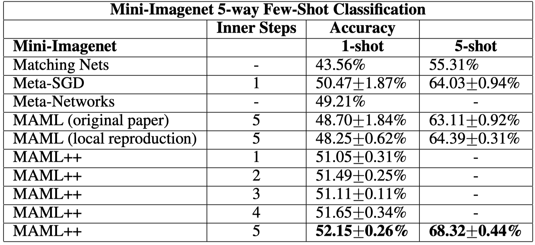
Then we show MAML++ on Mini-Imagenet tasks
References
- Antreas, Antoniou, Harrison Edwards, and Amos Storkey. 2019. “How To TrainYour MAML.” ICLR, 1–11.
- Code: https://github.com/AntreasAntoniou/HowToTrainYourMAMLPytorch
- Zhenguo Li et al. Meta-sgd: Learning to learn quickly for few shot learning.
- Ilya Loshchilov and Frank Hutter. SGDR: Stochastic Gradient Descent with Warm Restarts

