
Introduction
Recurrent neural networks, such as LSTM, often serve as memory for solving partially observable environments, where certain amount of information is concealed from the sensor of the agent. However, Wayne et al. 2018 show that memory is not enough; it is critical that the right information be stored in the right state. As a result, they develop a model, called Memory, RL, and Inference(MERLIN), in which memory formation is guided by a process of predictive modeling.
Method
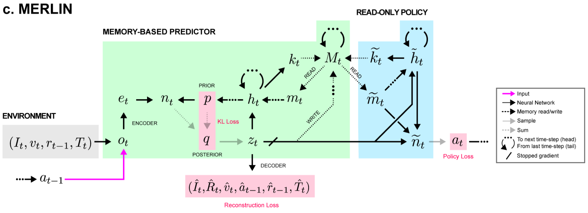
MERLIN consists of the memory-based predictor(MBP) and the policy. The MBP contains an external memory that stores a history of state variables. The policy takes as input the state variable and also reads from the external memory.
Overview
At each time step, the MBP first encodes environment information and computes the prior distribution from the outputs of the MBP LSTM at the previous time step. All these outputs are then concatenated and used to compute the posterior distribution, from which we compute a state variable \(z_t\). At last, we construct a set of reconstruction decoders, a policy, a value function, and an advantage function based on \(z_t\).
Memory-Based Predictor
We can roughly regard the MBP as a sequential VAE with an external memory, which consists of three parts: an encoder, an external memory, and a decoder. In the rest of this section, we briefly discuss each part in turn.
Encoder
MBP takes as inputs whatever information is available, including the previous action and reward. In particular, images are encoded by a ResNet, texts are passed through a LSTM, and velocity are processed by a linear layer. Actions and rewards are left as they are. These encodings are then concatenated into a flat vector \(e_t\).
Deocder
MBP reconstructs all inputs through respective decoders. Besides that, it further predicts the return using two networks. The first network takes in the concatenation of the latent variable, which we will discuss later, with the policy distribution’s multinomial logits \([z_t, \log\pi(a_t\vert M_{t-1},z_{\le t})]\), and returns a state value \(V^\pi_t=V^\pi(z_t,\log\pi_t)\). The second network takes in the concatenation \([z_t,a_t]\) and outputs a state-action advantage \(A^\pi(z_t,a_t)\). These two quantities are then added together to produce a return prediction, which could be regarded as a state-action value, \(\hat R_t^\pi=\text{StopGradient}(V_t^\pi)+A_t^\pi\). Notice that the gradients are not back-propagated through the value function, as it has its own loss function.
Memory
The memory system is based on a simplification of the Differentiable Neural Computer(DNC). The memory is a two-dimensiontal matrix \(M_t\) of size \((N, 2\times\vert z\vert )\), where \(\vert z\vert \) is the dimensionality of the the latent state vector sampled from the posterior distribution(see discussion below). The memory at the beginning of each episode is initialized blank, i.e., \(M_0=0\). Unlike DNC, MERLIN augments the memory by additionally storing a representation of events that occured after it in time, called retroactive memory updating. This is implemented by doubling the dimensionality of the rows, which now stores a concatenation of state variable \(z_t\) and a discounted sum of future state variables: \([z_t,(1-\gamma)\sum_{t’>t}\gamma^{t’-t}z_{t’}]\), with the discount factor \(\gamma<1\).
MBP LSTM
Both MBP and policy contain a deep LSTM of two hidden layers. The LSTM of MBP receives concatenated input \([z_t,a_t,m_{t-1}]\), where \(z_t\) is the latent state, \(a_t\) is the one-hot representation of the action, and \(m_{t-1}= [m_{t-1}^1, \dots, m_{t-1}^{K^r}]\) is a list of \(K^r\) vectors read from the memory at the previous time step. The LSTM produces an ouput \(h_t=[h_t^1,h_t^2]\), the concatenation of the output from each layer. A linear layer is applied to the output, and a memory interface vector \(i_t\) of dimension \(K^r\times(2\times \vert z\vert +1)\) is constructed. \(i_t\) is then segmented into \(K^r\) read vectors \(k_t^1,\dots,k_t^{K^r}\) of length \(2\times \vert z\vert \) and \(K^r\) scalars which are passed through a softplus function \(\text{softplus}(x)=\log(1+\exp(x))\) to create read strengths \(\beta_t^1,\dots,\beta_t^{K^r}\)
Reading
As in DNC, reading is content-based whose weights are computed based on the cosine similarity between each read key and each memory row
\[\begin{align} w^i(M, k^i,\beta^i)[j]={\exp(\beta^i c(k^i,M[i,\cdot]))\over\sum_j\exp(\beta^i c( k^i,M[j,\cdot]))}\\\ c[u,v]={u\cdot v\over |u||v|} \end{align}\]where \(k^i\) is a read key, \(\beta^i\) is the corresponding read strength, and \(c[u,v]\) computes the cosine similarity between \(u\) and \(v\).
Writing
After reading, writing to memory occurs. There are two types of writing. The first simply store the latent variable \(z_t\) to the \(i\)-th row of memory, which is achieved by a delta write weighting \(v_t^{w}[i]=\delta_{it}\in[0,1]^{\vert M\vert \times 1}\). The second weighting for retroactive memory updates is the moving average of the first
\[\begin{align} v_t^{ret}=\gamma v_{t-1}^{ret}+(1-\gamma)v_{t-1}^w \end{align}\]where \(\gamma\) is the same as the discount factor for the task. Notice that the delta write weighting at the previous step is used above, which ensures the second part of the memory only stores information after it in time.
Given these two weighting, the memory update can be written as an online update
\[\begin{align} M_t=M_{t-1}+v_t^w[z_t,0]^\top+v_t^{ret}[0,z_t]^\top \end{align}\]where \([z_t,0]^\top\) and \([0,z_t]^\top\) are of shape \([1, 2\times\vert z\vert ]\) with \(z_t\) in the beginning/end. Thus, \(v_t^w[z_t,0]^\top\) writes \(z_t\) to the first half of a chosen row; and \(v_t^{ret}[0,z_t]^\top\) adds \((1-\gamma)z_t\) to all previously written rows.
In case the number of memory rows is less than the episode length, overwriting of rows is necessary. To implement this, each row \(k\) contains a usage indicator: \(u_t[k]\). This indicator is initialized to \(0\) until the row is first written to. Subsequently, the row’s usage is increased if the row is read from by any of the reading heads \(u_{t+1}[k]=u_t[k]+\sum_iw_{t+1}^i[k]\). When allocating a new row for writing, the row with smallest usage is chosen.
Prior Distribution
The prior distribution is produced by an MLP that takes in the output from the MBP LSTM at the previous time step \([h_{t-1}, m_{t-1}]\) and produces a diagonal Gaussian distribution \(\mu_t^{prior},\log\Sigma_t^{prior}\).
Post Distribution
The posterior distribution is produced in two stages. First, we concatenates the outputs of all the encoders, the output of the MBP LSTM, and the prior distribution
\[\begin{align} n_t=[e_t,h_{t-1},m_{t-1},\mu_t^{prior},\log\Sigma_t^{prior}] \end{align}\]Note that \(h_{t-1}\) and \(m_{t-1}\) is from the previous time step, which makes sense as we rely on the previous information to make decision.
This vector is then propagated through an MLP that produces an output \(f^{post}(n_t)\) of size \(2\times \vert z\vert \). The output of this MLP is added to the prior distribution to determine the posterior distribution: \([\mu_t^{post},\log\Sigma_t^{post}]=f^{post}(n_t)+[\mu_t^{prior},\log\Sigma_t^{prior}]\).
State Variable Generation
The state variable is sampled from the posterior distribution using the reparameterization tricks.
Policy
The policy also contains a deep LSTM that read from the memory in the same way as the MBP, but using only one read key, giving outputs \([\tilde h_t,\tilde m_t]\). These outputs are then concatenated again with the latent variable \([z_t,\tilde h_t,\tilde m_t]\) and passed through an MLP that produces probability distribution for the action. The action \(a_t\) is sampled and passed to the MBP LSTM as an additional input, as described before.
Losses
The MBP is updated following the ELBO to errors of the decoders. We leave the details to the paper for interested readers as the decoders are environment specific. We only stress the return and policy losses here. The return loss is two folds:
\[\begin{align} \mathcal L_{return}={1\over 2}\left(\Vert R_t-V^\pi(z_t,\log\pi_t)\Vert^2+\Vert R_t-(\text{StopGradient}(V^\pi(z_t,\log\pi_t))+A^\pi(z_t,a_t))\Vert^2\right)_t \end{align}\]The policy gradient loss is updated with the Generalized Advantage Estimation algorithm:
\[\begin{align} \mathcal J=\sum_{t=k\tau}^{(k+1)\tau}\sum_{t'-t}^{(k+1)\tau}(\gamma\lambda)^{t'-t}\delta_{t'}\log\pi(a_t|h_t) \end{align}\]Where we truncate episodes into segments of length \(\tau\).
References
Wayne, Greg, Chia-Chun Hung, David Amos, Mehdi Mirza, Arun Ahuja, Agnieszka Grabska-Barwinska, Jack Rae, et al. 2018. “Unsupervised Predictive Memory in a Goal-Directed Agent.” http://arxiv.org/abs/1803.10760.