
Spectral Norm
Three equivalent definitions of the spectral norm of a matrix \(\pmb A\), \(\sigma(\pmb A)\):
- It is the largest singular value of \(\pmb A\), or equivalently, it is the square root of the largest eigenvalue of the product \(\pmb A^\top\pmb A\).
- It is the maximum, over all nonzero vectors \(\pmb{x} \in \mathbb R^n\), of the quotients \(\frac{\vert \pmb A\pmb{x} \vert }{\vert \pmb{x} \vert }\) where \(\vert \cdot \vert \) denotes the Euclidean norm.
- It is the maximum of the Euclidean norms of vectors \(\pmb A\pmb x\) where \(\pmb x\) is on the unit sphere, i.e., has Euclidean norm 1.
Proof: From (1), we can get that the spectral norm of \(\pmb A\) is the square root of the largest solution \(\lambda\) to \(\pmb A^\top\pmb A\pmb x=\lambda \pmb x\). Multiplying both sides of the identity by \(\pmb x^\top\) and take the square, we have
\[\begin{align} \sqrt{\pmb x^\top\pmb A^\top\pmb A\pmb x}&=\sqrt{\pmb x^\top\lambda \pmb x}\\\ &=\sqrt{\lambda \pmb x^\top\pmb x}\\\ \Rightarrow\sqrt \lambda&=\sqrt{\pmb x^\top\pmb A^\top\pmb A\pmb x\over \pmb x^\top \pmb x}\\\ &=\frac{\| \pmb A\pmb{x} \|}{\| \pmb{x} \|}\tag {1} \end{align}\]Therefore, we have \(\sigma(\pmb A)=\sqrt{\lambda_{\max}}=\max \frac{\vert \pmb A\pmb{x} \vert }{\vert \pmb{x} \vert }\), where \(\pmb x\in \mathbb R^n, \pmb x\ne \pmb0\), which gives us \((2)\). In the above analysis, we implicitly assume \(\pmb x\) is an eigenvector of the linear transformation. This does not need to be the case as \(\pmb A^\top \pmb A\) is a symmetric metric and we can derive \(\lambda_\max=\max_{\Vert \pmb x\Vert\ne 0}{\pmb x^\top\pmb A\pmb x\over \pmb x^\top\pmb x}\) following the Rayleigh-Ritz theorem. \((3)\) simply normalizes \(\pmb x\), therefore the denominator of Equation \((1)\) becomes \(1\) and we have \(\sigma(\pmb A)=\max\Vert \pmb A\pmb x\Vert\), where \(\Vert\pmb x\Vert=1\).
Connection with Lipschitz Norm for Linear Functions
Define a linear function \(f(\pmb x)=\pmb A\pmb x\). We say \(f(\pmb x)\) is K-Lipschitz continuous if for all \(\pmb x\) and \(\pmb x’\),
\[\begin{align} \Vert f\Vert_{Lip}={\Vert f(\pmb x)-f(\pmb x')\Vert\over \Vert \pmb x-\pmb x'\Vert}\le K\\\ \end{align}\]where \(\Vert\cdot\Vert\) is the \(\ell_2\) norm and we say \(\Vert f\Vert_{Lip}\) is the Lipschitz norm of \(f\) following Miyato et al 2018. It is easy to see the connection between the Lipschitz and the spectral norm of \(f\) once we rewrite \(\Vert f\Vert_{Lip}\)
\[\begin{align} \Vert f\Vert_{Lip}=\max_{\pmb \delta}{\Vert \pmb A\pmb \delta\Vert\over\Vert\pmb \delta\Vert}=\sigma(\pmb A)\\\ where\quad\pmb \delta=\pmb x-\pmb x' \end{align}\]Spectral Norm Regularization
Yoshida et al. 2017 propose to regularize networks by restricting the spectral norm of the weight matrices. They shows that if all activation functions are piecewise linear(e.g. ReLU), to achieve a flat local minimum, it is sufficient to bound the spectral norm of the weight matrix at each layer.
Considering a network \(f_\theta\) parameterized by \(\theta\), we want it to be robust to small perturbation \(\pmb \delta\) to the input \(\pmb x\). Therefore, we define the metric as the \(\ell_2\)-norm of \(f_\theta(\pmb x+\delta)-f_\theta(\pmb x)\). If we assume all activations are piecewise linear(e.g. ReLU), then \(f_\theta\) is a piecewise linear function and locally we can take regard \(f_\theta\) as a linear function. This allows us to represent \(f\) locally by an affine map \(\pmb x\mapsto W_{\theta,\pmb x}\pmb x+\pmb b_{\theta,\pmb x}\), for a small perturbation to the input, we have
\[\begin{align} {\Vert f_\theta(\pmb x+\pmb \delta)-f_\theta(\pmb x)\Vert_2\over \Vert\pmb \delta\Vert_2}={\Vert W_{\theta,\pmb x}(\pmb x+\pmb \delta)+\pmb b_{\theta,\pmb x})-(W_{\theta,\pmb x}\pmb x+\pmb b_{\theta,\pmb x})\Vert_2\over \Vert\pmb \delta\Vert_2}={\Vert W_{\theta,\pmb x}\pmb \delta\Vert_2\over \Vert\pmb \delta\Vert_2}\le \sigma(W_{\theta,\pmb x}) \end{align}\]where \(\sigma(W_{\theta,\pmb \delta})\) is the spectral norm of \(W_{\theta, \pmb\delta}\).
Notice that the above analysis is based on a strong assumption that \(f_\theta(\pmb x+\pmb \delta)\) lies in the linear neighbor of \(f_\theta(\pmb x)\). We assume it is true in this post. Let’s denote the activation at layer \(l\) as a local diagonal matrix \(D_{\theta,\pmb x}^l\) and weight in each layer as \(W^l\). We can rewrite \(W_{\theta,\pmb x}\) as \(W_{\theta,\pmb x}=\prod_{l=1}^LD_{\theta,\pmb x}^lW^l\). Notice tha \(\sigma(D_{\theta,\pmb x}^l)\le 1\) for all \(l\in{1,\dots,L}\). Hence we have
\[\begin{align} \sigma(W_{\theta,\pmb x})\le \prod_{l=1}^L\sigma(D_{\theta,\pmb x}^l)\sigma(W^l)\le\prod_{l=1}^L\sigma(W^l) \end{align}\]It follows that, to bound the spectral norm of \(W_{\theta,\pmb x}\), it suffices to bound the spectral norm of \(W^l\) for each \(l\in {1,\dots,L}\). We do not discuss the regularization method proposed by Yoshida et al. 2017, which manually tackles the gradients of each layer. Instead, we briefly mention several take-aways from the paper next, and discuss another method for regularizing spectral norm in the next section.
Several take-aways
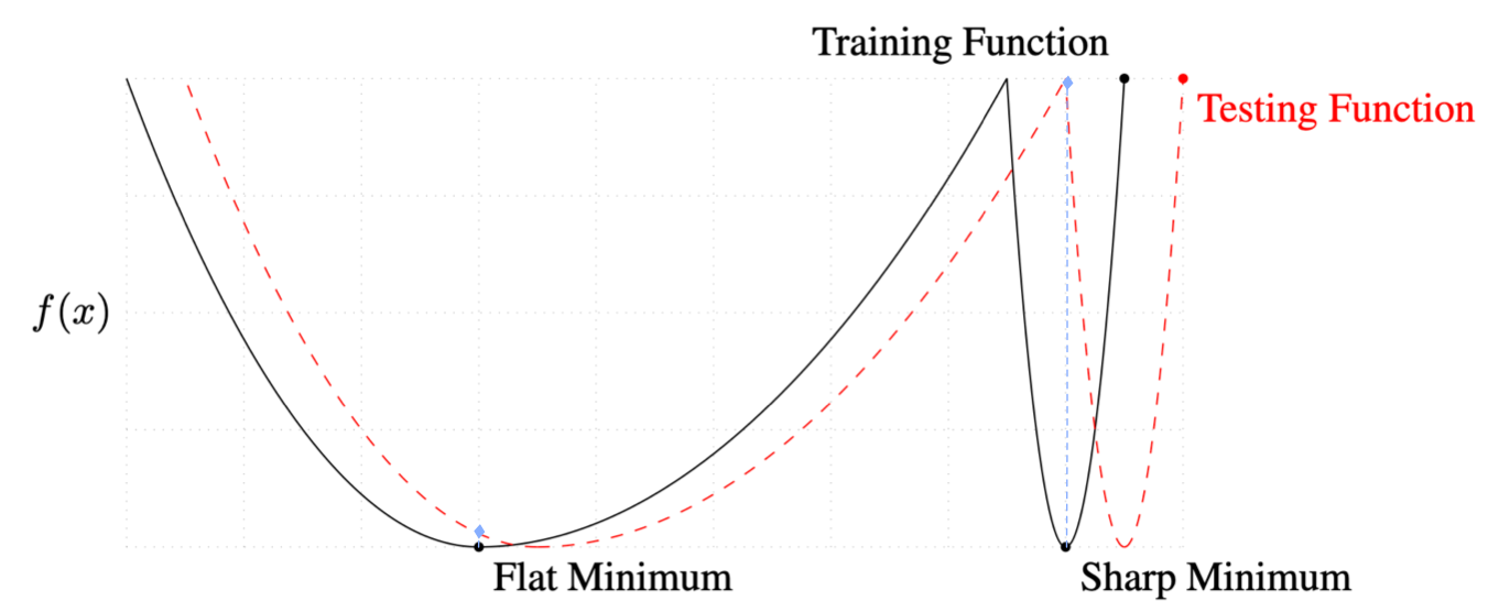
- Hochreiter&Jurgen Schmidhuber 1997 shows A flat local minimum generalizes better than a sharp one (see Figure 1 for an illustration).
- Keskar et al. 2017 shows SGD with smaller minibatch size tends to converge to a flatter minimum.
- Goodfellow et al. 2015 shows that training using adversarial examples improves test accuracy.
- Arjovsky et al. and Wisdom et al shows that by restricting the weight matrices in RNN to be unitary or orthogonal, the problem of diminishing/exploding gradients in RNN can be prevented and better performance can be obtained.
Spectral Norm Layers
Based on Yoshida et al. 2017, Miyato et al. 2018 develope spectral normalization layers, which explicitly normalizes the spectral norm of the weight matrix in each layer so that it satisfies the Lipschitz constraints \(\sigma(W)=1\):
\[\begin{align} W_{SN}(W):=W/\sigma(W) \end{align}\]where \(\sigma(W)\) is the spectral norm of \(W\). We can verify its spectral norm by showing
\[\begin{align} \sigma(W_{SN}(W))=\sigma(W)/\sigma(W)=1 \end{align}\]Miyato et al. 2018 further prove that spectral normalization regularizes the gradient of \(W\), preventing the column space of \(W\) from concentrating into one particular direction. This precludes the transformation of each layer from becoming sensitive in one direction.
How to Compute The Spectral Norm?
Assume \(W\) is of shape \((N, M)\) and we have a randomly initialized vector \(u\). The power iteration method computes the spectral norm of \(W\) as follows
\[\begin{align} &\mathbf{For}\ i= 1...T:\\\ &\quad v = W^Tu/\Vert W^Tu\Vert_2\\\ &\quad u = Wv/\Vert Wv\Vert_2\\\ &\sigma(W)=u^TWv \end{align}\]where \(u\) and \(v\) approximate the first left and right singular vector of \(W\). In practice, \(T=1\) is sufficient since we gradually update \(W\) as well.
References
Yuichi Yoshida and Takeru Miyato. Spectral norm regularization for improving the generalizability of deep learning
Sepp Hochreiter and Jurgen Schmidhuber. Flat minima. Neural Computation, 9(1):1–42, 1997.
Nitish Shirish Keskar, Dheevatsa Mudigere, Jorge Nocedal, Mikhail Smelyanskiy, Ping Tak Peter Tang. On large-batch training for deep learning - generalization gap and sharp minima. In ICLR, 2017.
Ian J. Goodfellow, Jonathon Shlens, Christian Szegedy. Explaining and Harnessing Adversarial Examples. In ICLR 2015
Martin Arjovsky, Amar Shah, Yoshua Bengio. Unitary evolution recurrent neural networks. In ICML, pages 1120–1128, 2016.
Scott Wisdom, Thomas Powers, John R. Hershey, Jonathan Le Roux, Les Atlas. Full-capacity unitary recurrent neural networks. In NIPS, pages 4880–4888, 2016.
Takeru Miyato, Toshiki Kataoka, Masanori Koyama, Yuichi Yoshida. Spectral normalization for generative adversarial networks. In ICLR 2018
Supplementary Materials
Rayleigh-Ritz theorem
Rayleigh-Ritz theorem: Let \(\pmb A \in \mathbb R^{n\times n}\) be a symmetric matrix. Then its eigenvectors are the critical points of the Rayleigh quotient defined as
\[\begin{align} R(\pmb x)={\pmb x^\top\pmb A^\top\pmb A\pmb x\over \pmb x^\top \pmb x} \end{align}\]As a consequence, we have
\[\begin{align} \lambda_{\max}=\max_{\Vert\pmb x\Vert\ne 0}{\pmb x^\top\pmb A^\top\pmb A\pmb x\over \pmb x^\top \pmb x} \end{align}\]and
\[\begin{align} \lambda_{\min}=\min{\Vert\pmb x\Vert\ne 0}{\pmb x^\top\pmb A^\top\pmb A\pmb x\over \pmb x^\top \pmb x} \end{align}\]Proof. At the critic point \(\bar{\pmb x}\), we have
\[\begin{align} {dR(\bar{\pmb x})\over d \bar{\pmb x}}={d({\bar{\pmb x}^\top\pmb A^\top\pmb A\bar{\pmb x}\over \bar{\pmb x}^\top \bar{\pmb x}})\over d\bar{\pmb x}}\pmb 0 \end{align}\]Using the derivative rule, we obtain
\[\begin{align} { {(\bar{\pmb x}^\top\pmb A^\top\pmb A\bar{\pmb x})\over d\bar{\pmb x}}\bar{\pmb x}^\top \bar{\pmb x} -\bar{\pmb x}^\top\pmb A^\top\pmb A\bar{\pmb x} {d(\bar{\pmb x}^\top \bar{\pmb x})\over d\bar{\pmb x}} \over (\bar{\pmb x}^\top \bar{\pmb x})^2}&=\pmb 0\\\ { {(\bar{\pmb x}^\top\pmb A^\top\pmb A\bar{\pmb x})\over d\bar{\pmb x}} -R(\bar{\pmb x}) {d(\bar{\pmb x}^\top \bar{\pmb x})\over d\bar{\pmb x}} \over \bar{\pmb x}^\top \bar{\pmb x}}&=\pmb 0\\\ 2\pmb A\bar{\pmb x}-2R(\bar{\pmb x})\bar{\pmb x}&=0\\\ \pmb A\bar{\pmb x}&=R(\bar{\pmb x})\bar{\pmb x} \end{align}\]The proof complete as the last equation is the eigenvalue equation.