
Introduction
We discuss Neural Turing Machine, an architecture proposed by Graves et al. 2014. NTMs are designed to solve tasks that require writing to and retrieving information from an external memory, which makes it resemble a working memory system that can be described by short-term storage(memory) of information and its rule-based manipulation. Compared with RNN structure with internal memory, NTMs utilize attentional mechanisms to efficiently read and write an external memory, which makes them a more favorable choice for capturing long-range dependencies. But, as we will see, these two are not independent of each other and can be combined to form a more powerful architecture.
Neural Turing Machines
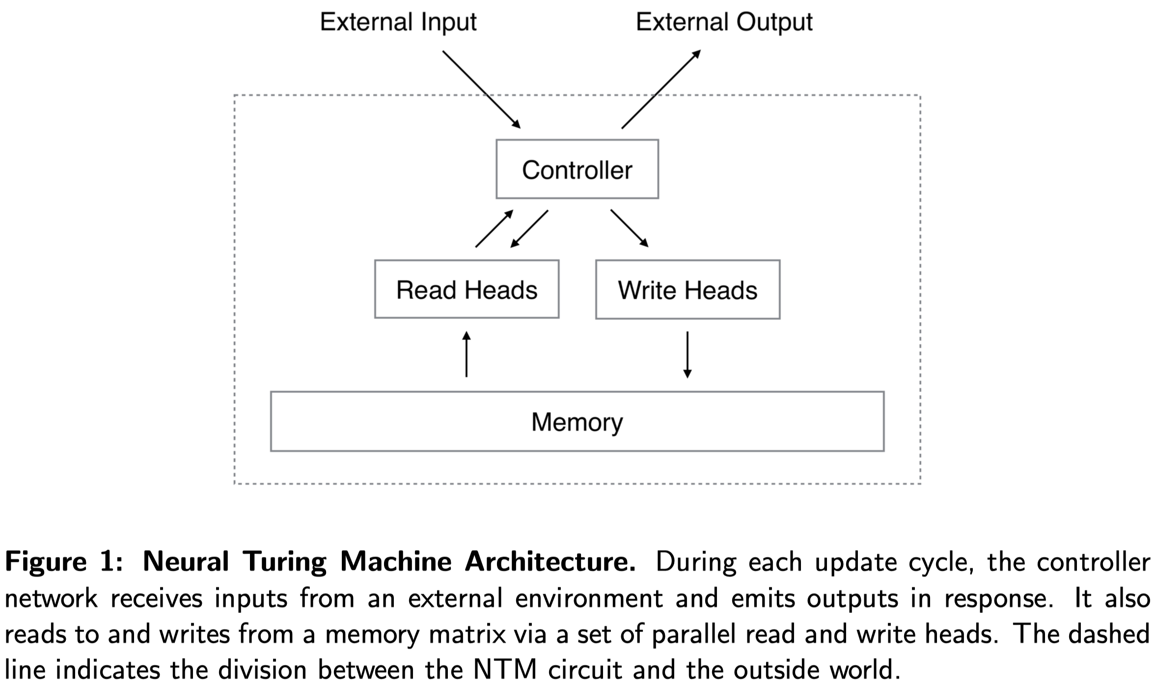
The overall architecture of NTM is demonstrated in Figure 1. The controller is a general neural network, an MLP or RNN, which receives inputs and previous read vectors and omits outputs in response. In addition, it reads to and writes from a memory matrix via a set of parallel read and write heads. The memory is an \(N\times W\) matrix, where \(N\) is the number of memory locations(rows), and \(W\) is the vector size at each location.
Reading
At each time step \(t\), a read head outputs a vector \(\pmb w_t\) of normalized weightings over the \(N\) locations. The read vector \(\pmb r_t\) of length \(W\) returned by the head is defined as a weighted combination of the row-vectors \(\pmb M_t(i)\):
\[\begin{align} \pmb r_t=\sum_iw_t(i)\pmb M_t(i)\\\ s.t.\quad\sum_i w_t(i)=1 \end{align}\]We can vectorize the above equation
\[\begin{align} \pmb r_t=\pmb M_t^{\top}\pmb w\tag{1} \end{align}\]Writing
The write is decomposed into two parts: an erase followed by an add. At each time step \(t\), a write head emits three vectors: an \(N\)-dimensional weighting vector \(\pmb w_t\), a \(W\)-dimensional erase vector \(\pmb e_t\), and a \(W\)-dimensional add vector \(\pmb a_t\). Each memory vector \(\pmb M_{t-1}(t)\) is modified first by the erase vector:
\[\begin{align} \tilde {\pmb M}_t(i)= \pmb M_{t-1}(i)[\pmb 1-w_t(i)\pmb e_t] \end{align}\]where \(\pmb 1\) is a row-vector of all 1-s, and the multiplication against the memory location acts point-wise. Then the add vector applies
\[\begin{align} \pmb M_t(i)=\tilde {\pmb M}_t(i)+w_t(i)\pmb a_t \end{align}\]We can also combine the above two operations and vectorize them as follows
\[\begin{align} \pmb M_t=\pmb M_{t-1}\circ(\pmb E-\pmb w_t\pmb e_t^{\top})+\pmb w_t\pmb v_t^{\top}\tag{2} \end{align}\]Addressing Mechanisms
So far, we have shown the equations of reading and writing, but we haven’t described how the weightings are produced. These weightings arise by combining two addressing mechanisms with complementary facilities:
- The first mechanism, content-based addressing, focuses attention on locations based on their similarity to weightings emitted by the controller. It could be an attention mechanism built on cosine similarity which we have seen back when we discussed Transformer.
- The second mechanism, location-based addressing, recognizes variables based on their locations instead of content. This mechanism is essentially useful for arithmetic problems: e.g., variables \(x\) and \(y\) can take on any values, but as long as their address is recognized, the procedure \(f(x,y)=x\times y\) should still be defined.
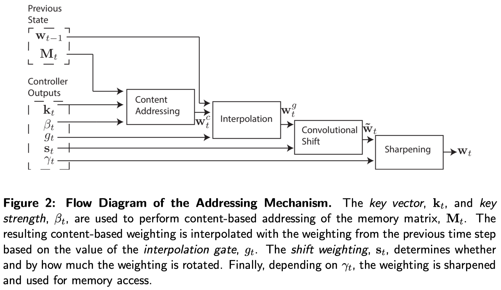
Notice that content-based addressing is strictly more general than location-based addressing as the content of a memory location could include location information inside it. In experiments, however, Graves et al. found providing location-based addressing as a primitive operation proved essential for some forms of generalization, therefore they employed both mechanisms concurrently. Figure 2 demonstrate the whole addressing mechanism. We will walk through it step by step in the following sub-sections
Content-Based Addressing
For content-addressing, we compute a normalized weighting \(\pmb w_t^c\) based on the cosine similarity between rows of \(\pmb M_t\) and a \(W\)-dimensional key vector \(\pmb k_t\). In order to tune the effectiveness of the cosine similarity, we additionally introduce a positive key strength \(\beta_t\), which can amplify or attenuate the precision of focus. This results in the following weighting
\[\begin{align} w_t^c(i)&={\exp(\beta_tK[\pmb k_t,M_t(i))])\over\sum_j\exp(\beta_tK[\pmb k_t, M_t(i))]}\\\ K[\pmb u,\pmb v]&={\pmb u\cdot\pmb v\over \Vert\pmb u\Vert\Vert\pmb v\Vert} \end{align}\]we could vectorize this computation as
\[\begin{align} \pmb w_t^c=\text{softmax}(\beta_t\tilde{\pmb M}_t\tilde{\pmb k}_t)\tag{3} \end{align}\]where \(\hat {\pmb M}\) is \(\pmb M\) with \(\ell^2\)-normalized rows and \(\hat{\pmb k}\) is \(\ell^2\)-normalized \(\pmb k\).
Location-Based Addressing
The location-based addressing mechanism is designed to facilitate both simple iterations across the locations of the memory and random-access jumps. It does so by implementing a rotational shift of a weighting.
Prior to the rotation, each head emits a scalar interpolation gate \(g_t\) in the range \((0, 1)\). The value of \(g_t\) is used to blend between the weighting \(\pmb w_{t-1}\) produced by the head at the previous time step and the content-based weighting \(\pmb w_t^c\):
\[\begin{align} \pmb w_t^g\leftarrow g_t\pmb w_t^c+(1-g_t)\pmb w_{t-1}\tag {4} \end{align}\]Especially when \(g_t=0\), \(\pmb w_t^g\) equals to \(\pmb w_{t-1}\), which completely omits the content-based weighting and simply focus on location shift.
After interpolation, we apply to the weighting a 1-D convolutional shift kernel, whose parameters \(\pmb s_t\) are a normalized categorical distribution produced by the head with zero-padding if necessary(see code in the end for example):
\[\begin{align} \tilde w_t(i)\leftarrow\sum_{j=0}^{N-1}w_t^g(j)s_t(i-j)\tag {5} \end{align}\]where all index arithmetic is computed modulo \(N\). This convolution operation can cause leakage or dispersion of weightings over time if the shift weighting \(\pmb s_t\) is not sharp. To combat this, each head emits one further scalar \(\gamma_t\ge 1\) whose effect is to sharpen the final weighting as follows:
\[\begin{align} w_t(i)\leftarrow{\tilde w_t(i)^{\gamma_t}\over\sum_j\tilde w_t(j)^{\gamma_t}}\tag {6} \end{align}\]Noticeably, as Graves et al. mentioned in experiments, they found Equation \((4)\) and Equation \((6)\) play a nontrivial role in generalizing NTM beyond the range of training data.
Summaries
Now we summarize the addressing mechanism as follows:
- Compute the content weighting \(\pmb w_t^c\) using Equation \((3)\).
- Compute the gated weighting \(\pmb w_t^g\) by interpolating content weighting \(\pmb w_t^c\) into the previous weighting \(\pmb w_{t-1}\), which is done by Equation \((4)\).
- Apply the 1D convolutional kernel to the gated weighting to get a local-based weighting \(\tilde {\pmb w}_t\) following Equation \((5)\).
- Compute the final weighting by sharpening \(\tilde{\pmb w}_t\) using Equation \((6)\).
The combined addressing system of weighting interpolation and content and location-based addressing can operate in three complementary modes:
- A weighting can be chosen by the content system without any modification by the location system, in which case we have \(g_t=1, s_t(0)=1,s_t(j)=0\text{ for }j\ne 0, \gamma_t=1\).
- A weighting produced by the content addressing system can be chosen and then shifted. This allows the focus to jump to a location next to, but not on, an address accessed by content; in computational terms, this allows a head to find a contiguous block of data, then access a particular element within that block
- A weighting from the previous time step can be rotated without any input from the content-based addressing system(\(g_t=0\)). This allows the weighting to iterate through a sequence of addresses by advancing the same distance at each time-step.
For those with CS background, we can draw an analogy between the addressing system and pointers in C/C++: the content system instructs the initial location the pointer points to, and the location system further moves the pointer around that location.
Implementation
In this section, we further discuss some implementation details from the work of Collier&Beel.
Memory Contents Initialization
They tried three different memory content initialization:
- Constant initialization: all memory locations are initialized to \(10^{-6}\)
- Learned initialization: we backpropagate through memory initialization at training time
- Random initialization: Each memory location is initialized to a value drawn from a truncated Normal distribution with mean \(0\) and standard deviation \(0.5\).
They found constant initialization works much better than the other two schemes.
Other Parameter Initialization
They backpropagate through the initialization of read vectors \(\pmb r_0\) and address weights \(\pmb w_0\) instead of initializing them to bias values.
Similarity Measure
They use cosine similarity as Equation \((3)\) suggests
Controller Inputs
At each time step \(t\), the controller receives the input coming from the environment and read vectors \(\pmb r_{t-1}\) from all of the read heads of the NTM.
Parameter non-linearities
They apply
- the tanh function to key vector \(\pmb k_t\) and add vector \(\pmb a_t\)
- the sigmoid function to the erase vector \(\pmb e_t\) and gate \(g_t\)
- the softplus function to key strength to satisfy the constraint \(\beta_t>0\)
- the softmax function to convolutional shift vector \(\pmb s_t\)
- the oneplus function(\(\mathrm{oneplus}(x)=1+\log(1+e^x)\)) to sharpen factor \(\gamma_t\)
Code for Equation \((5)\)
s = tf.concat(
  [s[:, :shift_range + 1],
  tf.zeros([s.get_shape()[0], memory_size - (shift_range * 2 + 1)]),
  s[:, -shift_range:]], axis=1
)
t = tf.concat([tf.reverse(s, axis=[1]), tf.reverse(s, axis=[1])], axis=1)
s_matrix = tf.stack(
    [t[:, memory_size - i - 1: memory_size * 2 - i - 1]
     for i in range(memory_size)],
    axis=1
)
w_ = tf.reduce_sum(tf.expand_dims(w_g, axis=1) * s_matrix, axis=2)     # equation (5)
Let’s take a simple example to see this process more clearly. Assume that the memory size(i.e., \(N\)) is \(4\), shift range is \(1\), and \(s=[0.5, 0.2,0.3]\), where \(0.5\) is the center mass(For the sake of simplicity, we omit the batch dimension here). Then we have
w_g = np.array([
  [.1, .2, .3, .4]
])
s = np.array([.5, .2, 0, .3])
t = np.array([.3, 0, .2, .5, .3, 0, .2, .5])
s_matrix = np.array([
  [.5, .3, 0, .2],
  [.2, .5, .3, 0],
  [0, .2, .5, .3],
  [.3, 0, .2, .5]
])
w_ = np.sum(w_g * s_matrix, axis=1)
# >>> array([0.19, 0.21, 0.31, 0.29])
References
Alex Graves, Greg Wayne, and Ivo Danihelka. 2014. “Neural Turing Machines,” 1–26. http://arxiv.org/abs/1410.5401.
Collier, Mark, and Joeran Beel. 2018. “Implementing Neural Turing Machines.” Lecture Notes in Computer Science (Including Subseries Lecture Notes in Artificial Intelligence and Lecture Notes in Bioinformatics) 11141 LNCS: 94–104. https://doi.org/10.1007/978-3-030-01424-7_10.