
Introduction
Recurrent Neural Networks(RNNs), Long Short-Term Memory(LSTM) and Gated Recurrent Units(GRU) in particular, have been firmly established as state-of-the-art approaches in sequence modeling and transduction problems. Such models typically rely on hidden states to maintain historical information. This is beneficial in that it allows the model to make predictions based on useful historical information distilled in the hidden state. On the other hand, this inherently sequential nature precludes parallelization, which becomes critical at longer sequence lengths, as memory constraints limit batching across examples. Furthermore, in these models, the number of operations required to relate signals from two arbitrary input or output positions grows in the distance between positions, which makes it more difficult to learn dependencies between distant positions.
In this post, we will discuss a model named Transformer, proposed by Vaswani et al. in 2017, which utilizes self-attention to compute representations of its input and output without using sequence-aligned RNNs. In this way, it reduces the number of operations required to relate signals from two arbitrary positions to a constant number and achieves significantly more parallelization. Note that, here we only try to illustrate the main architecture of the model and the central idea of attention. For other NLP-related details, please refer to [1] and [2].
One thing may be worth keeping in mind is that the Transformer we introduce here maintains sequential information in a sample just as RNNs do. This suggests the input to the network is of form [batch size, sequence length, embedding size]. In many RL literature, the sequential dimension is usually replaced by an entity dimension. As a result, the network can learn to attend to some entity that related to the agent’s current state.
Model Architecture
The Transformer follows the encoder-decoder structure using stacked self-attention and fully connected-layers for both the encoder and decoder, shown in the left and right halves of the following figure, respectively
Positional Encoding
In sequential forecast, it is important to incorporate positional information so that the network learns how to predict based not only on the past events but also on the order of these events. However, neither the self-attention modules nor fully-connected layers exploits the input order. To tip off the network the relative position of the input in the sequence, we introduce positional encoding to explicitly incorporate positional information into the input. Specifically, we use sine and cosine functions of different frequencies to encode the position information into a \(d_{model}\)-dimensional feature:
\[\begin{align} PE_{(pos, 2i)}&=\sin(pos/10000^{2i/d_{model}})\\\ PE_{(pos, 2i+1)}&=\cos(pos/10000^{2i/d_{model}}) \end{align}\]where \(pos\) is the token’s position in the sequence and \(i\) is the embedding dimension. That is, each dimension of the positional embedding corresponds to a sinusoid. The wavelengths form a geometric progression from \(2\pi\) to \(10000⋅2\pi\). We chose this function because we hypothesized it would allow the model to easily learn to attend by relative positions, since for any fixed offset \(k\), \(PE_{pos+k}\) can be represented as a linear function of \(PE_{pos}\) (Proof in Supplementary Materials).
Encoder and Decoder Stacks
Encoder
The encoder is composed of a stack of \(N=6\) identical layers. Each layer has two sublayers. The first is a multi-head self-attention mechanism, and the second is a simple fully connected feed-forward network. Residual connections are employed around each of the two sub-layers, and layer normalization is applied in between. Mathematically, we denote the output of each sub-layer as \(x+\mathrm{Sublayer}(\mathrm{LayerNorm}(x))\) (This one, adopted by [2], is slightly different from the one used in the paper, but follows the pattern standard residual networks recommend), where \(\mathrm{Sublayer}(x)\) is the function implemented by the sub-layer itself.
Decoder
The decoder is also composed of a stack of \(N=6\) identical layers. In addition to the two sub-layers in the encoder layer, the decoder inserts a third sub-layer, which performs multi-head attention over the output of the encoder stack (i.e., where we have the output of the encoder as keys and values). Sub-layers in the decoder follows the same fashion as that in the encoder.
Masking
Masks are used before softmax in the self-attention layer in both encoder and decoder to prevent unwanted attention to out-of-sequence positions. Furthermore, in conjunction with the general mask, an additional mask is used in the self-attention sub-layers in the decoder stack to prevent positions from attending to subsequent positions. Such masks have the form of
\[\begin{align} \begin{matrix} 1&0&0&\dots&0\\\ 1&1&0&\dots&0\\\ 1&1&1&\dots&0\\\ \vdots&\vdots&\vdots&\ddots&\vdots\\\ 1&1&1&\dots&1 \end{matrix} \end{align}\]In practice, the two masks in the decoder can be blended via a bit-wise and operation.
Attention
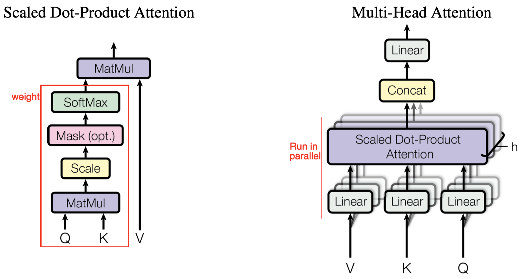
Scaled Dot-Product Attention
An attention function can be described as a mapping from a query and a set of key-value pairs to an output, where the query, keys, values, and output are all vectors. The output is computed as a weighted sum of the values, where the weight assigned to each value is computed by a compatibility function of the query with the corresponding key:
\[\begin{align} \mathrm{Attention}(Q,K,V)=\mathrm{softmax}\left(QK^T\over\sqrt{d_k}\right)V \end{align}\]where \(Q, K, V\) are queries, keys, and values, respectively; \(d_k\) is the dimension of the keys; the compatibility function (softmax part) computes the weights assigned to each value in a row. The dot-product \(QK^T\) is scaled by \(1\over \sqrt{d_k}\) to avoid extremely small gradients for large values of \(d_k\), where the dot-product grows large in magnitude, pushing the softmax function into the edge region. In the resulting matrix \(A\), the features in the rows are the weighted sum of features in \(V\), i.e., \(A_{i,:}=\sum_k w_{i,k}V_{k,:}\), where \(w_{i,k}\) explains the similarity between \(Q_i\) and \(K_k\).
Multi-Head Attention
Single attention head averages attention-weighted positions, reducing the effective resolution. Multi-head attention allows the model to jointly attend to information from different representation subspaces at different positions. For example, when two positions \(k_1,k_2\) are highly related to position \(i\). In the single-head attention, the output averages values at \(k_1, k_2\), blurring the effect of values. In the multi-head attention, the network may learn to attend to \(k_1, k_2\) in two different heads.
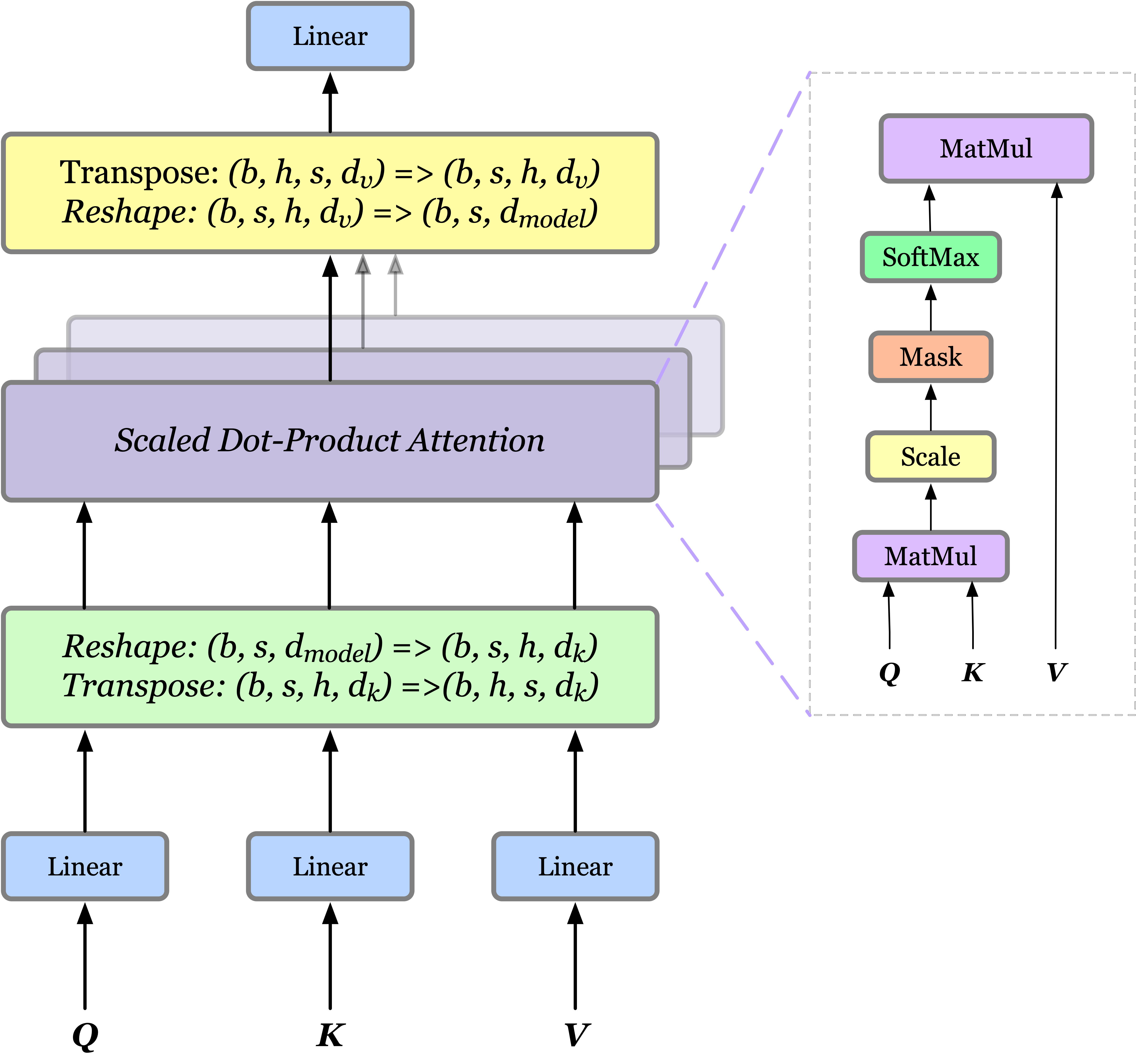
Mathematically, multi-head attention is expressed as follows
\[\begin{align} \text{MultiHead}(Q,K,V)&=\mathrm{Concat}(\mathrm{head}_1,\dots,\mathrm{head}_h)W^O\\\ where\ \text{head}_i &=\text{Attention}(QW_i^Q,KW_i^K,VW_i^V) \end{align}\]where the projections are parameter matrices \(W_i^Q\in\mathbb R^{d_{\mathrm{model}}\times d_k}\), \(W_i^K\in\mathbb R^{d_{\mathrm{model}}\times d_k}\), \(W_i^V\in\mathbb R^{d_{\mathrm{model}}\times d_v}\) and \(W^O\in\mathbb R^{hd_v\times d_{\mathrm{model}}}\). For each head, we first apply a fully-connected layer to reduce the dimension, then we pass the result to a single attention function. At last, all heads are concatenated and once again projected, resulting in the final values. Since all heads run in parallel and the dimension of each head is reduced beforehand, the total computational cost is similar to that of single-head attention with full dimensionality.
In practice, if we have \(hd_k=hd_v=d_{model}\), multi-head attention can be simply implemented using attention with four additional fully-connected layers, each of dimension \(d_{model}\times d_{model}\) as follows
Tensorflow Code
class MultiHeadSelfAttention(layers.Layer):
    def __init__(self,
                 key_size,
                 val_size,
                 num_heads,
                 scale_logits=True,
                 out_size=None,
                 pre_norm=False,
                 norm='layer',
                 norm_kwargs={},
                 drop_rate=0,
                 use_rezero=False,
                 name="sa",
                 **kwargs):
        super().__init__(name=name)
        self._key_size = key_size
        self._val_size = val_size
        self._num_heads = num_heads
        self._scale_logits = scale_logits
        self._out_size = out_size
        self._pre_norm = pre_norm
        self._norm = norm
        self._norm_kwargs = norm_kwargs
        self._drop_rate = drop_rate
        self._use_rezero = use_rezero
        kwargs.setdefault('use_bias', False)
        self._kwargs = kwargs

    def build(self, input_shape):
        assert len(input_shape) == 3, input_shape
        seqlen, out_size = input_shape[1:]
        qkv_size = 2 * self._key_size + self._val_size
        total_size = qkv_size * self._num_heads
        out_size = self._out_size or out_size

        prefix = f'{self.name}/'
        self._embed = layers.Dense(total_size, **self._kwargs, name=prefix+'embed')
        self._att = Attention(prefix+'att')

        self._group_heads = layers.Reshape((seqlen, self._num_heads, qkv_size), name=prefix+'group_heads')
        self._concat = layers.Reshape((seqlen, self._num_heads * self._val_size), name=prefix+'concat')
        self._out = layers.Dense(out_size, **self._kwargs, name=prefix+'out')
        if self._drop_rate > 0:
            self._drop = layers.Dropout(self._drop_rate, (None, None, 1), name=prefix+'drop')

        norm_cls = get_norm(self._norm)
        self._norm_layer = norm_cls(**self._norm_kwargs, name=prefix+self._norm)
        if self._use_rezero:
            self._rezero = tf.Variable(0., trainable=True, dtype=tf.float32, name=prefix+'rezero')

        super().build(input_shape)

    def call(self, x, training=False, mask=None):
        y = call_norm(self._norm, self._norm_layer, x, training) \
            if self._pre_norm else x
        qkv = self._embed(y)
        qkv = self._group_heads(qkv)                    # [B, N, F] -> [B, N, H, F/H]
        qkv = tf.transpose(qkv, [0, 2, 1, 3])           # [B, N, H, F/H] -> [B, H, N, F/H]

        q, k, v = tf.split(qkv, [self._key_size, self._key_size, self._val_size], -1)

        # softmax(QK^T/(d**2))V
        if self._scale_logits:
            q *= self._key_size ** -.5
        out = self._att(q, k, v, mask)
        # equivalence using einsum
        # dot_product = tf.einsum('bqhf,bkhf->bqhk', q, k)
        # if mask is not None:
        #     dot_product *= mask
        # weights = tf.nn.softmax(dot_product)
        # out = tf.einsum('bqhk,bkhn->bqhn', weights, v)

        # [B, H, N, V] -> [B, N, H, V]
        out = tf.transpose(out, [0, 2, 1, 3])
        # [B, N, H, V] -> [B, N, H * V]
        y = self._concat(out)
        y = self._out(y)

        if self._drop_rate > 0:
            y = self._drop(y, training=training)
        if self._use_rezero:
            y = self._rezero * y
        x = x + y
        x = x if self._pre_norm else \
            call_norm(self._norm, self._norm_layer, x, training)

        return x
References
Ashish Vaswani et al. Attention Is All You Need
Guillaume Klein et al. OpenNMT: Open-Source Toolkit for Neural Machine Translation
Timo Denk. Linear Relationships in the Transformer’s Positional Encoding.
Supplementary Materials
Proof that \(PE_{i+k}\) is a linear function of \(PE_{i}\)
Rewrite \(PE_i\) as follows
\[\begin{align} PE_i=& \begin{bmatrix} \sin(a_1i)&\cos(a_1 i)&\dots&\sin(a_ni)&\cos(a_ni) \end{bmatrix}^\top\\\ where\quad a_j=&{1\over10000^{2j/d_{model}}},\quad n=d_{model}/2 \end{align}\]We show that there exits a linear map \(T^{k}\) such that \(T^kPE_i=PE_{i+k}\). More specifically, \(T^k\) can be expressed as the following matrix
\[\begin{align} T^k=& \begin{bmatrix} \pmb \Phi_1^k&\pmb 0&\dots&\pmb 0\\\ \pmb 0&\pmb \Phi_2^k&\dots&\pmb 0\\\ \vdots&\vdots&\ddots&\vdots\\\ \pmb 0&\pmb 0&\dots&\pmb \Phi_n^k \end{bmatrix}\\\ where\quad \pmb \Phi_j^k=& \begin{bmatrix} \cos(a_jk)&\sin(a_jk)\\\ -\sin(a_jk)&\cos(a_jk) \end{bmatrix} \end{align}\]With these notations, we now show \(T^kPE_i=PE_{i+k}\), i.e.,
\[\begin{align} \pmb \Phi_j^k\begin{bmatrix}\sin(a_ji)\\\\cos(a_ji)\end{bmatrix}=\begin{bmatrix}\sin(a_j(i+k))\\\\cos(a_j(i+k))\end{bmatrix} \end{align}\]for all \(j\in[0,d_{model/2}]\).
Expanding \(\pmb \Phi_j^k\), we have
\[\begin{align} \pmb \Phi_j^k\begin{bmatrix}\sin(a_ji)\\\\cos(a_ji)\end{bmatrix}=& \begin{bmatrix} \cos(a_jk)&\sin(a_jk)\\\ -\sin(a_jk)&\cos(a_jk) \end{bmatrix} \begin{bmatrix}\sin(a_ji)\\\\cos(a_ji)\end{bmatrix}\\\ =&\begin{cases} \cos(a_jk)\sin(a_ji)+\sin(a_jk)\cos(a_ji)\\\ \cos(a_jk)\cos(a_ji)-\sin(a_jk)\sin(a_ji)\\\ \end{cases}\\\ &\qquad\color{red}{\text{apply the angle addition formula}}\\\ =&\begin{cases} \sin(a_j(i+k))\\\ \cos(a_j(i+k)) \end{cases}\\\ =&\begin{bmatrix}\sin(a_j(i+k))\\\\cos(a_j(i+k))\end{bmatrix} \end{align}\]