
Introduction
Many combinations of RNN architectures and attention mechanisms, such as RMC and DNC, have been covered in this blog. In this post, we first briefly review the content-based input attention proposed by Bahdanau et al.. Then we shift our attention to pointer network(PtrNet) proposed by Vinyals&Fortunato.
Content-Based Input Attention
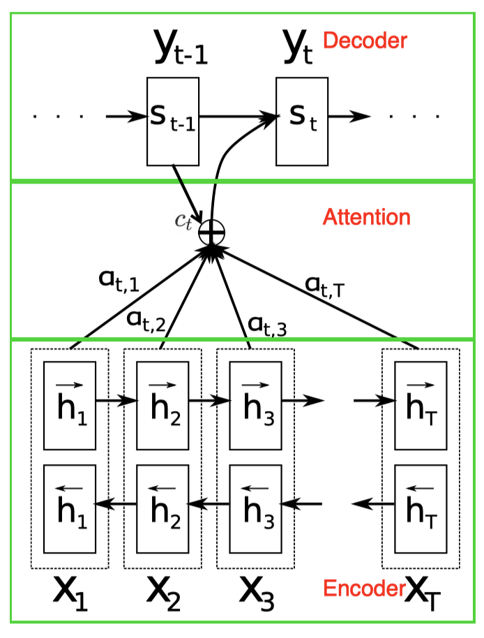
Traditional seq2seq models produce the entire output sequence using the fixed dimensional state of the recognition RNN at the end of the input sequence. This constrains the amount of information that computation can flow through to the generative model. Bahdanau et al. 2015 proposed to add an additional attention model to ameliorate this problem so that the model can learn to attend to different parts of the input sequence for different outputs. In particular, they use a bidirectional LSTM as the recognition network that encodes all sequential information. The generative network is another RNN that predicts the output \(s_t\) for the current time-step based on the previous hidden state \(s_{t-1}\) and the current context vector \(c_t\) from the encoder. Mathematically, we have
\[\begin{align} p(s_t|s_1,\dots,s_{t-1},\mathbf x)&=f(s_{t-1}, c_t) \end{align}\]where \(f\) denotes an RNN operation, and the context vector \(c_t\) depends on a sequence of annotations \(h_1, \dots, h_T\) to which an encoder maps the input sequence. Each annotation \(h_t\) contains information about the whole input sequence with a strong focus on the parts surrounding the \(t^{th}\) element of the input sequence. In practice, an annotation \(h_t\) is the concatenation of hidden states computed by the forward and backward RNNs.
The context vector \(c_t\) is computed as a weighted sum of these annotations
\[\begin{align}c_t&=\sum_{k=1}^Ta_{tk}h_k\\\where\quad a_{tk}&=\mathrm {softmax}(f_{att}(s_{t-1}, h_k))\end{align}\]Intuitively, \(c_t\) is computed through an attention module where the weight \(a_{tk}\) of \(h_k\) is associated to the similarity between \(s_{t-1}\) and \(h_k\). Introducing \(s_{t-1}\) in the attention function \(f_{att}\) gives the freedom to the decoder to decide to which parts of the source sentence to pay attention based on it’s previous state.
The attention function \(f_{att}\) calculates an unnormalized alignment score that reflects the importance of the annotation \(h_k\) with respect to the previous hidden state \(s_{t-1}\) in deciding the next state \(s_t\) and generating \(y_t\). It’s typically defined as one of the following
\[\begin{align} f_{att}(s_{t-1}, h_k)=\begin{cases} s_{t-1}^{\top}h_k&\text{dot}\\\ s_{t-1}^{\top}Wh_k&\text{general}\\\ v^{\top}\tanh(W_ss_{t-1}+W_hh_k)&\text{concat} \end{cases} \end{align}\]where \(v^\top\) is a column of the weights in a dense layer.
Pointer Network
While the above model serves the needs of translating an input sequence into an output sequence, such as machine translation, the pointer network(PtrNet) is targeted at selecting a sequence of members of the input sequence as the output, e.g., finding planar convex hulls or solving the planar Traveling Salesman Problem. As a result, PtrNet can be concisely expressed as follow
\[\begin{align} u_{t,k}&=f_{att}(s_{t-1}, h_k)\\\ p(s_t|s_1,\dots,s_{t-1},\mathbf x)&=\text{softmax}(u_{t,k}) \end{align}\]where \(\mathbf x\) is the input position, \(f_{att}=v^\top\tanh(W_s s_{t-1}, W_h h_k)\) is the concat attention. The decoder computes the similarity between the encoder state \(h_k\) and decoder state \(s_{t-1}\). Unlike the previous attention-based seq2seq model, we do not further blend \(h_k\) into the output with an attention weight as the output is associated to the input position but not the content.
Another appealing property of PtrNet is that it’s able to deal with a varying-length output. This is because we use the same attention module to compute all \(u_{t,k}\).
Inference
Another worth mentioning part of these seq2seq algorithms is the beam search method used at inference time.
Notice that selecting the most probable value at each step during inference is likely to get a suboptimal solution because the output probabilities are dependent. However, maximizing the sequential probability \(p(s_{1:T_{out}}\vert h_{1:T_{in}})\) is computationally intractable because of the combinatorial number of possible output sequences. As a result, we usually use a beam search procedure to find the best possible sequence given a beam size \(n\), which repeats the following steps for each time step
- At each time step \(t\), we maintain \(n\) subsequences \(s_{1:t-1}\) from the previous step, each with its probability \(p(s_{1:t-1}\vert h_{1:T_{in}})\).
- Then for each \(s_{1:t-1}\), we compute all \(p(s_t\vert h_{1:T_{in}}, s_{1:t-1})\) and multiply them by \(p(s_{1:t-1}\vert h_{1:T_{in}})\) to get \(p(s_{1:t}\vert h_{1:T_{in}})=p(s_{1:t-1}\vert h_{1:T_{in}})p(s_t\vert h_{1:T_{in}},s_{1:t-1})\).
- We then select new \(n\) subsequences \(s_{1:t}\) with the maximal probabilities \(p(s_{1:t}\vert h_{1:T_{in}})\) for the next stage.
References
Oriol Vinyals, Meire Fortunato, Navdeep Jaitly. Pointer Networks
Dzmitry Bahdanau, KyungHyun Cho, Yoshua Bengio. Neural Machine Translation by Jointly Learning to Align and Translate