
Introduction
We discuss Ape-X DQfD, proposed by Pohlen et al. 2018, that combines the following techniques into Ape-X DQN:
- Transformed Bellman operator that allows the algorithm to process rewards of varying densities and scales for deterministic environments.
- Temporal consistency loss that allows us to train stably using a large discount factor \(\gamma=0.999\) (instead of \(\gamma=0.99\) in traditional DQN) extending the effective planning horizon by an order of magnitude
- DQfD that uses human demonstrations to guide the agent towards rewarding states so as to ease the exploration problem
Transformed Bellman Operator
Mnih et al. 2015 have empirically observed that the errors introduced by the limited network capacity, the approximate finite-time solution to the loss function, and the stochasticity of the optimization problem can cause the algorithm to diverge if the variance/scale of the action-value function is too high. In order to reduce the variance, they clip the reward distribution to the interval \([-1, 1]\). While this achieves the desired goal of stabilizing the algorithm, it significantly changes the set of optimal policies. Instead of clipping the reward, Pohlen et al. proposed to reduce the scale of the action-value function using the transformed Bellman operator defined below
\[\begin{align} \mathcal T_h(Q)(x,a)&:=\mathbb E_{x'\sim P(\cdot|x,a)}\left[h\left(R(x,a)+\gamma\max_{a'\in\mathcal A}h^{-1}(Q(x',a'))\right)\right]\\\ where\quad h(z)&=\text{sign}(z)(\sqrt{|z|+1}-1)+\epsilon z, \epsilon=10^{-2} \end{align}\]where the additive regularization term \(\epsilon z\) ensures that \(h^{-1}\) is Lipschitz continuous. This \(h\) is chosen because it has the desired effect of reducing the scale of the targets while being Liptschitz continuous and admitting a closed form inverse (see Supplementary Materials for details). The temporal difference loss is thus defined as
\[\begin{align} L_{TD}(\theta)=\mathbb E[\mathcal L((\mathcal T_hQ_{\theta^-})(x,a)-Q_\theta(x,a))] \end{align}\]where \(\mathcal L\) is the huber loss, and \(\theta^-\) denotes the target network parameters.
The experiments show the transformed Bellman operator improves the performance compared to one with the standard Bellman operator and PopArt, which adaptively rescales the targets for the value network to have zero mean and unit variance.
Temporal Consistency Loss
As \(\gamma\) approaches \(1\), the temporal difference in value between non-rewarding states becomes negligible. This can be seen from
\[\begin{align} Q(x,a) - Q(x',a')&=R(x,a)-(1-\gamma)Q(x',a')\\\ &=(1-\gamma)Q(x',a'),\quad \text{when }R(x,a)=0 \end{align}\]When reward is zero and \(\gamma\) approaces \(1\), the temporal difference becomes \(0\).
Similar results were also observed by Durugkar and Stone that due to over-generalization in DQN, updates to the value of the current state have an adverse effect on the value of the next state, resulting in unstable learning when the discount factor is high. Pohlen et al. addressed this using the temporal consistency loss, which penalize the changes in the next action-value estimate
\[\begin{align} L_{TC}(\theta)=\mathbb E[\mathcal L(Q_\theta(x',a')-Q_{\theta^-}(x',a'))] \end{align}\]where \(\theta^-\) is the network parameter before applying SGD. This TD loss penalizes weight updates that change the next action-value estimate \(Q(x’,a’)\). The experiments show that the TC loss is paramount to learning stably with higher \(\gamma\). They spot that without TC loss, the algorithm learns faster at the beginning of the training process. However, at some point during training, the performance collapses and often the process dies with floating point exceptions.
DQfD
To utilize expert data, it uses the same imitation loss from DQfD defined as a max-margin loss of the form
\[\begin{align} L_{IM}(\theta)=\mathbb E\left[e\left(\max_{a_i\in\mathcal A}[Q_\theta(x,a_i)+\lambda\delta_{a_i\ne a}]-Q_\theta(x,a)\right)\right] \end{align}\]where \(e\) is the an indicator that is \(1\) if the transition is from the best expert episode(i.e., with the highest score) and \(0\) otherwise, \(\lambda\in\mathbb R\) is the margin and \(\delta_{a_i\ne a}\) is \(1\) if \(a_i\ne a\) and \(0\) otherwise. This loss forces the values of the other actions to be at least a margin lower than the value of the demonstrator’s action. Adding this loss grounds the value of the unseen actions to reasonable values, and makes the greedy policy induced by the value function imitate the demonstrator.
Ape-X DQfD
The following figure demonstrates the architecture of Ape-X DQfD, there is nothing new here.
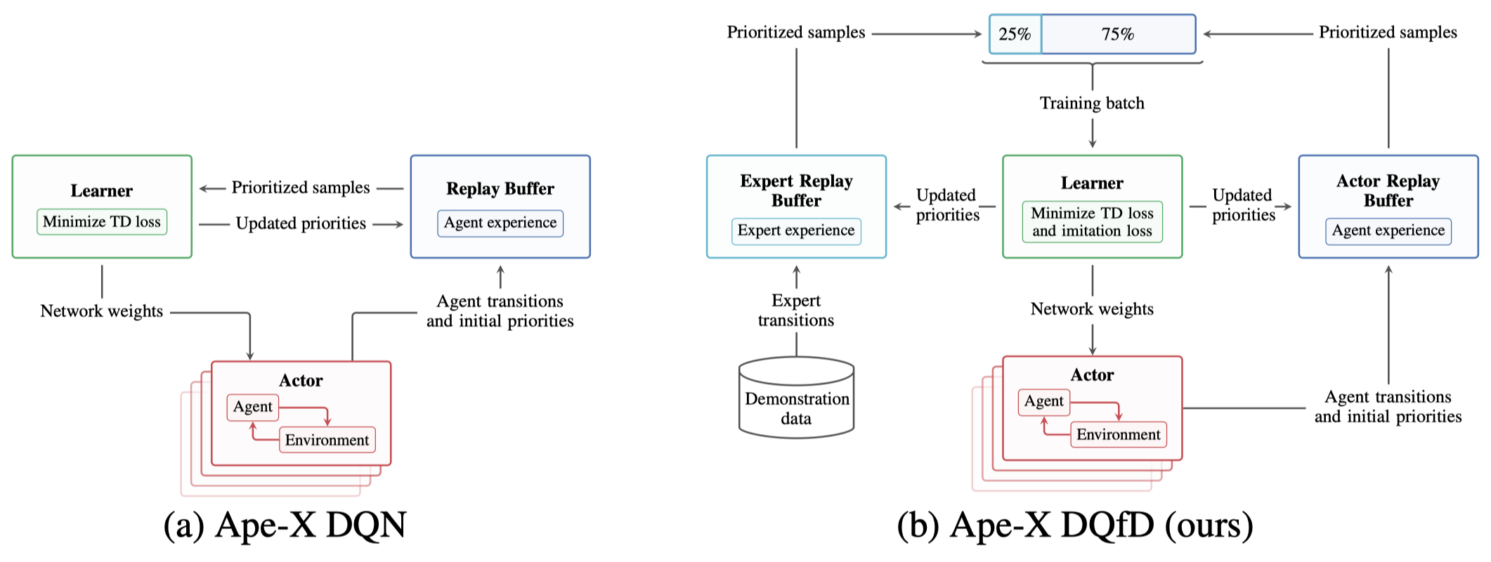
Noticeably, the expert data significantly improves the performance on sparse reward games but impairs the performance on games where the agent can effectively explore.
Takeaways from Experimental Results
Some takeaways from their experimental results:
- Jiang et al. 2015 argue that A large \(\gamma\) increases the complexity of the learning problem and, thus, requires a bigger hypothesis space. Hence, Pohlen et al. increase the capacity of the network architecture and spot improvements on performance
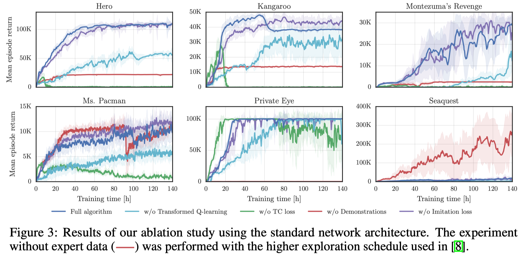
From Figure 3, we can see that
- The transformed Bellman operator significantly improves the overall performance.
-
TC loss is paramount to learning stably with \(\gamma=0.999\). Without the TC loss, the algorithm learns faster in the beginning, but at some point during the training, the performance collapses and the process often dies with floating point exceptions
- Demonstrations are especially helpful in environments with sparse reward but they impair the performance on dense reward environments
References
- Tobias Pohlen, Bilal Piot, Todd Hester, Mohammad Gheshlaghi Azar, Dan Horgan, David Budden, Gabriel Barth-Maron, Hado van Hasselt, John Quan, Mel Vecerík, Matteo Hessel, Rémi Munos, and Olivier Pietquin. Observe and Look Further: Achieving Consistent Performance on Atari
- Ishan Durugkar and Peter Stone. TD learning with constrained gradients. In Deep Reinforcement Learning Symposium, NIPS, 2017.
- Hado van Hasselt, Arthur Guez, Matteo Hessel, Volodymyr Mnih, and David Silver. Learning values across many orders of magnitude. In Proc. of NIPS, 2016.
- Volodymyr Mnih, Koray Kavukcuoglu, David Silver, Andrei A. Rusu, Joel Veness1, Marc G. Bellemare, Alex Graves, Martin Riedmiller, Andreas K. Fidjeland, Georg Ostrovski, Stig Petersen, Charles Beattie, Amir Sadik, Ioannis Antonoglou, Helen King, Dharsha, Shane Legg & Demis Hassabis. 2015. “Human-Level Control through Deep Reinforcement Learning.” *Macmillan Publishers.
- Nan Jiang, Alex Kulesza, Satinder Singh, and Richard Lewis. The dependence of effective planning horizon on model accuracy. In Proceedings of the 2015 International Conference on Autonomous Agents and Multiagent Systems, pages 1181–1189. International Foundation for Autonomous Agents and Multiagent Systems, 2015.
Supplementary Materials
Property of \(h(x)\)
We here justify the transformed Bellman operator; we show that the choice of \(h(x)=\text{sign}(x)(\sqrt{\vert x\vert +1}-1)+\epsilon x\) has the following property:
- \(h\) is strictly monotonically increasing
- \(h\) is Lipschitz continuous with Lipschitz constant \(L_h={1\over 2}+\epsilon\)
- \(h\) is invertible with \(h^{-1}(x)=\text{sign}(x)\left(\left({\sqrt{1+4\epsilon(\vert x\vert +1+\epsilon)}-1\over2\epsilon}\right)^2-1\right)\)
- \(h^{-1}\) is strictly monotonically increasing
- \(h^{-1}\) is Lipschitz continuous with Lipschitz constant \(L_{h^{-1}}={1\over\epsilon}\)
We first introduce the following two Lemmas:
**Lemma 1: **\(h(x)=\text{sign}(x)(\sqrt{\vert x\vert +1}-1)+\epsilon x\) is differentiable everywhere with derivative \({d\over dx}h(x)={1\over 2\sqrt{\vert x\vert +1}}+\epsilon\).
Lemma 2: \(h^{-1}(x)=\text{sign}(x)\left(\left({\sqrt{1+4\epsilon(\vert x\vert +1+\epsilon)}-1\over2\epsilon}\right)^2-1\right)\) is differentiable everywhere with derivative \({d\over dx}h^{-1}(x)={1\over\epsilon}\left(1-{1\over\sqrt{1+4\epsilon(\vert x\vert +1+\epsilon)}}\right)\).
We now prove all statements individually
-
We can prove that \({d\over dx}h(x)={1\over{2\sqrt{\vert x\vert +1}}}+\epsilon>0\) for all \(x\in\mathbb R\). Therefore, \(h\) is strictly monotonically increasing
-
Let \(x,y\in\mathbb R\) with \(x<y\), using the mean value theorem, we find
-
1 implies \(h\) is invertible and \(h\circ h^{-1}(x)=h^{-1}\circ h(x) = x\) proves \(h^{-1}\) is \(h\)’s inverse
-
Because \({d\over dx}h^{-1}(x)={1\over\epsilon}\left(1-{1\over\sqrt{1+4\epsilon(\vert x\vert +1+\epsilon)}}\right)>0\) for all \(x\in\mathbb R\), \(h^{-1}\) is strictly monotonically increasing
-
Let \(x,y\in\mathbb R\) with \(x<y\), using the mean value theorem, we find
Contraction
The authors did not prove that \(\mathcal T_h\) is a contraction in stochastic domain. Instead, they proved that \(\mathcal T_h\) is a contraction when \(h\) is strictly monotonically increasing and the MDP is deterministic: Let \(Q^*\) be the fixed point of \(\mathcal T\), we have
\[\begin{align} h\circ Q^\*&=h\circ\mathcal TQ^\*\\\ &=h\circ\mathcal T(h^{-1}\circ h\circ Q^\*)\\\ &=h\circ (R+\gamma \max_{a'} h^{-1}\circ Q^\*)\\\ &=\mathcal T_h(Q^\*) \end{align}\]where the last equation only holds because the MDP is deterministic