
Lipschitz Continuity
A function is Lipschitz continuous if there is a positive constant \(K\) such that, for all \(x\) and \(y\)
\[\begin{align} |f(x)-f(y)| < K|x-y| \end{align}\]This says the function \(f\) should not be sensitive the perturbation of its input up to a constant \(K\). Particularly, if the function is continuous, this says that the function has bounded derivative.
Furthermore, if the Lipschitz constant \(K<1\), the function \(f\) is a contraction.
Change of Variables
Single/Multiple Variables
Let \(X\in \mathbb R^n\) be a continuous multi-variate random variable, and let \(Y=f(X)\) be injective(one-to-one) and continuously differentiable. Then we have
\[\begin{align} dy=|\det(J_f(X))|dx \end{align}\]where \(\vert J_f(X)\vert \) is the Jacobian determinant. This is consistent with the single variable case where we have
\[\begin{align} dy=f'(x)dx \end{align}\]Application in Probability
Suppose we know the PDF of \(X\) as \(P(X)\), and let \(Y=f(X)\) be injective and continuously differentiable. Then we have
\[\begin{align} p_y(y)=p_x(x)\left|dx\over dy\right| \end{align}\]We prove this as follows: As \(f(X)\) is injective, geometrically, we have
\[\begin{align} |p_y(y)dy|=&|p_x(x)dx|\\\ \Longleftrightarrow\qquad p_y(y)=&p_x(x)\left |{dx\over dy}\right |\\\ \Longleftrightarrow\qquad p_y(y)=&p_x(x)\left|dy\over dx\right|^{-1} \end{align}\]where the equivalent is established because \(p_y(y),p_x(x)\ge0\).
In higher dimensions, the derivative generalizes to the determinant of the Jacobian matrix. Thus, we have
\[\begin{align} p_{\pmb y}(\pmb y)=p_{\pmb x}(\pmb x)\left|\det\left({d\pmb y\over d\pmb x}\right)\right|^{-1} \end{align}\]References
https://en.wikipedia.org/wiki/Integration_by_substitution#Substitution_for_multiple_variables
Duality Theorem
For a primal linear program defined by
\[\begin{align} &\text{maximize}&\pmb c^\top \pmb x\\\ &s.t. &\pmb A\pmb x\le \pmb b\\\ &&\pmb x\ge\pmb 0 \end{align}\]the dual takes the form
\[\begin{align} &\text{minimize}&\pmb b^\top \pmb y\\\ &s.t. &\pmb A^\top \pmb y\ge \pmb c\\\ &&\pmb y\ge\pmb 0 \end{align}\]This is called the symmetric dual problem. There are two other dual problems listed here. For simplicity, we only discuss the symmetric dual problem.
Weak Duality
Weak Duality: For any feasible solution \(x\) and \(y\) to primal and dual linear programs, \(\pmb c^\top \pmb x\le \pmb b^\top \pmb y\).
Proof: Multiplying both sides of \(\pmb A\pmb x\le \pmb b\) by \(\pmb y^\top\), we have \(\pmb y^\top \pmb A\pmb x\le \pmb y^\top \pmb b\). Since \(\pmb A^\top \pmb y\ge \pmb c\), we have \(\pmb c^\top \pmb x\le \pmb y^\top \pmb A\pmb x\le \pmb y^\top \pmb b\).
There are two immediate implication of weak duality:
- If both \(\pmb x\) and \(\pmb y\) are feasible solutions to the primal and dual and \(\pmb c^\top \pmb x=\pmb b^\top \pmb y\), then \(\pmb x\) and \(\pmb y\) must be optimal solutions
- If the optimal profit in the primal is \(\infty\), then the dual must be infeasible. If the optimal cost in the dual is \(-\infty\), then the primal must be infeasible
The weak duality always holds regardless whether the primal is convex or not.
Strong Duality
Strong Duality: The duality has an optimal solution if and only if the primal does. If \(\pmb x^*\) and \(\pmb y^*\) are optimal solutions to the primal and dual, then \(\pmb c^\top \pmb x^*=\pmb b^\top \pmb y^*\).
The strong duality only holds when the primal is convex.
To prove strong duality, we first introduce Farkas’ Lemma and KKT conditions.
Farkas’ Lemma
Farkas’ Lemma: Let \(\pmb A\in\mathbb R^{m⨉ n}\) and \(\pmb b\in\mathbb R^m\). Then exactly one of the following two assertions is true:
- There exists an \(\pmb x\in\mathbb R^n\) such that \(\pmb A\pmb x=\pmb b\) and \(\pmb x\ge 0\)
- There exists a \(\pmb y\in\mathbb R^m\) such that \(\pmb A^\top\pmb y\ge 0\) and \(\pmb b^\top\pmb y<0\)
Proof: If both \((1)\) and \((2)\) hold, then \(0>\pmb b^\top \pmb y=\pmb y^\top \pmb A\pmb x\ge 0\), which is a contradiction.
We resorts the following geometric interpretation to show that either \((1)\) or \((2)\) is true.
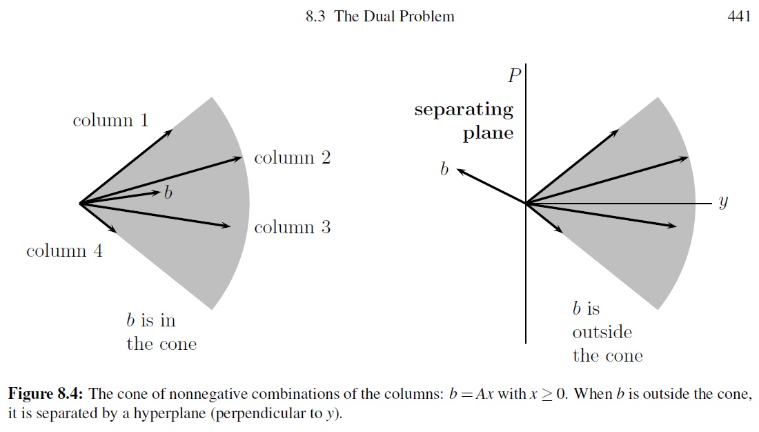
Geometric interpretation: Consider the closed convex cone spanned by the columns of \(\pmb A\); that is
\[\begin{align} C(\pmb A)=\{\pmb A\pmb x|\pmb x\ge 0\} \end{align}\]Farkas’ lemma equally says that either \(\pmb b\) in \(C(\pmb A)\) or there exists a hyperplane that separates \(\pmb b\) and \(C(\pmb A)\). If \(\pmb b\) is not in \(C(\pmb A)\), then we can compute \(\pmb y\) as the vector orthogonal to the hyperplane. The following figure visualizes these two cases
KKT conditions
KKT conditions: Suppose that \(f,g^1,g^2,g^M\) are differentiable functions from \(\mathbb R^N\) to \(\mathbb R\). Let \(\pmb x^*\) be the point that maximizes \(f\) subject to \(g^i(\pmb x)\le 0\) for each \(i\), and assume the first \(k\) constraints are active and \(\pmb x^*\) is regular. Then there exists \(\pmb y\ge 0\) such that \(\nabla f(\pmb x)=y_1\nabla g^1(\pmb x)+…+y_k\nabla g^k(\pmb x)\)
Proof: Let \(c=\nabla f(\pmb x^*)\). The directional derivative of \(f\) in the direction of vector \(\pmb z\) is \(\pmb z^\top\pmb c\). Because \(\pmb x^*\) is the maximum point, every feasible direction \(\pmb z\) must have \(\pmb z^\top\pmb c < 0\). Let \(\pmb A\in\mathbb R^{k\times N}\) be the matrix whose \(i\)th row is \((\nabla g^i(\pmb x))^\top\). Then a direction \(\pmb z\) is feasible if \(\pmb A\pmb z\le 0\). As \(\pmb z^\top\pmb c<0\) and \(\pmb A\pmb z\le 0\) violate Farkas’ case \((2)\) , there is a \(\pmb y\ge \pmb 0\) such that \(\pmb A\pmb y=\pmb c\).
Proof of Strong Duality
Let
\[\begin{align} \pmb{\hat A}=\begin{bmatrix}\pmb A\\\-\pmb I_n\\\-\pmb c^\top\end{bmatrix},\pmb{\hat b}=\begin{bmatrix}\pmb b\\\\pmb 0\\\-(\tau+\epsilon)\end{bmatrix} \end{align}\]where \(\tau=\pmb c^\top\pmb x^*\) is the optimal value of the primal, \(\epsilon\ge 0\) is an arbitrary value. Because \(\tau\) is the optimal value, there is no feasible \(\pmb x\) such that \(\pmb c^\top\pmb x=\tau+\epsilon\). Therefore, there is no \(\pmb x\in\mathbb R^n\) such that
\[\begin{align} \begin{bmatrix}\pmb A\\\-\pmb I_n\\\-\pmb c^\top\end{bmatrix}\pmb x\le \begin{bmatrix}\pmb b\\\\pmb 0\\\-(\tau+\epsilon)\end{bmatrix} \end{align}\]By the variant of Farkas’ Lemma, we have \(\pmb{\hat y}=\begin{bmatrix}\pmb y\\ \pmb z\\ \alpha\end{bmatrix}\ge0\), such that
\[\begin{align} \begin{bmatrix}\pmb y^\top&\pmb z^\top&\alpha\end{bmatrix} \begin{bmatrix}\pmb A\\\-\pmb I_n\\\-\pmb c^\top\end{bmatrix}=0,\quad \begin{bmatrix}\pmb y^\top&\pmb z^\top&\alpha\end{bmatrix}\begin{bmatrix}\pmb b\\\\pmb 0\\\-(\tau+\epsilon)\end{bmatrix}=-1\\\ \end{align}\]Thus, we have
\[\begin{align} \pmb y^\top\pmb A=\pmb z^\top+\alpha\pmb c^\top,\quad \pmb y^\top\pmb b=-1+\alpha(\tau+\epsilon)<\alpha(\tau+\epsilon) \end{align}\]If \(\alpha=0\), then the dual is unbounded or infeasible – for any feasible solution \(\pmb y_*\), we have \((\pmb y_*^\top+\lambda \pmb y^\top)\pmb A\ge\pmb c^\top+\lambda\pmb z^\top\) and \((\pmb y_*^\top+\lambda\pmb y^\top)\pmb b=\pmb y_*^\top\pmb b-\lambda\). Taking \(\lambda\) large, we see that the dual problem is unbounded. Therefore, \(\alpha>1\) and by scaling \(\pmb {\hat y}\), we may assume that \(\alpha=1\). So \(\pmb y^\top \pmb A\ge c^\top\) and \(\pmb y^\top\pmb b\le \tau+\epsilon\). By the Weak Dual Theorem, we have \(\tau= \pmb c^\top \pmb x\le\pmb y^\top\pmb b\le\tau+\epsilon\). Since \(\epsilon\) is arbitrary, we have \(\pmb c^\top \pmb x\le\pmb y^\top\pmb b\).
References
https://web.stanford.edu/~ashishg/msande111/notes/chapter4.pdf
http://www.ma.rhul.ac.uk/~uvah099/Maths/Farkas.pdf