
Introduction
General policy gradient methods face two main challenges: 1) stable and steady improvement despite the nonstationarity of incoming data; 2) sample efficiency. In the previous post, we have discussed TRPO and PPO which restrict the step size of policy updates to obtain a reliable improvement. In this post, we shift our focus to the second challenge, which is addressed by using value function to substantially reduce the variance of policy gradient estimates at cost of some bias, with exponentially-weighted estimator of the advantage function.
Table of Contents
Preliminary
First we introduce a notion of \( \gamma \)-just that will be frequently referred in the rest of the post. A \( \gamma \)-just estimator of the advantage function is an estimator that does not introduce bias when we use it to approximate the underlying real discounted advantage function \( A^{\pi,\gamma} \). In other word, an estimator is \( \gamma \)-just if \( \gamma \) is the only source of bias – recall that the discount factor \( \gamma \) could also be view as a variance reduction technique, at the price of some bias, as it diminishes the weight of future rewards. An estimator \( \hat A_t \) is \( \gamma \)-just for all \( t \) if
\[\begin{align} \mathbb E_{s_{0:\infty},a_{0:\infty}}\left[\hat A_t(s_{0:\infty}, a_{0:\infty})\nabla_\theta\log\pi_\theta(a_t|s_t)\right]=\mathbb E_{s_{0:\infty},a_{0:\infty}}\left[A^{\pi, \gamma}(s_t,a_t)\nabla_\theta\log\pi_\theta(a_t|s_t)\right]\tag{1} \end{align}\]where \(A^{\pi,\gamma}=Q^{\pi,\gamma}(s_t,a_t)-V^{\pi,\gamma}\) is the real discounted advantage function following policy \(\pi\).
One sufficient condition for \( \hat A_t \) to be \( \gamma \)-just is that
\[\begin{align} \hat A_t(s_{0:\infty}, a_{0:\infty})=Q_t(s_{t:\infty}, a_{t:\infty})-b_t(s_{0:t}, a_{0:t-1}) \tag{2} \end{align}\]where \( b_t \) is an arbitrary function of states and actions sampled before \( a_t \), and \( Q_t \), which can depend on any trajectory variables starting from \( s_t, a_t \), is an unbiased estimator of the discounted \( Q \)-function \( Q^{\pi,\gamma}(s_t,a_t) \), i.e.
\[\begin{align} \mathbb E_{s_{t+1:\infty}, a_{t+1:\infty}}\left[Q_t(s_{t:\infty}, a_{t:\infty})\right] = Q^{\pi, \gamma}(s_t, a_t) \end{align}\]detailed proof will be given in the end
Generalized Advantage Estimation
Let’s now consider the \( n \)-step advantage:
\[\begin{align} \hat A_t^{(n)} &= \sum_{i=0}^{n-1}r_{t+i}+\gamma^n V(s_{t+n})- V(s_t)\\\ &=r_{t}+\gamma V(s_{t+1})-V(s_{t})+\gamma\left(\sum_{i=1}^{n-1}r_{t+i+1 }+\gamma ^{n-1}V(s_{t+n})-V(s_{t+1})\right)\\\ &=\delta_t+\gamma\left(\sum_{i=0}^{n-2}r_{t+i+1}+\gamma ^{n-1}V(s_{t+n})-V(s_{t+1})\right)\\\ &=\sum_{i=0}^{n-1}\gamma^i\delta_{t+i}\tag{3} \end{align}\]Equation \((3)\) actually illustrates a very nice interpretation that if we view \( \delta_t \) as a shaped reward with \( V \) as the potential function (aka. potential-based reward), then the \( n \)-step advantage is actually \( \gamma \)-discounted sum of these shaped rewards. With this in mind, we further define the generalized advantage estimator \( GAE(\gamma, \lambda) \) as the exponentially-weighted average of all \( n \)-step estimators, which is closely analogous to \( TD(\lambda) \) in terms of advantage function:
\[\begin{align} \hat A_t^{GAE(\gamma, \lambda)}&:=(1-\lambda)\left(\sum_{n=0}^{\infty}\lambda^{n}\hat A_{t}^{(n+1)}\right)\\\ &=(1-\lambda)\left(\sum_{n=0}^{\infty}\lambda^n\sum_{i=0}^{n}\gamma^i\delta_{t+i}\right)\\\ &=(1-\lambda)\left(\sum_{i=0}^{\infty}\gamma^i\delta_{t+i}\sum_{n=i}^{\infty}\lambda^n \right)\\\ &=(1-\lambda) \left(\sum_{i=0}^{\infty}\gamma^i\delta_{t+i}\lambda^i\sum_{n=0}^{\infty}\lambda^n\right)\\\ &=(1-\lambda)\left(\sum_{i=0}^{\infty}(\gamma\lambda)^i\delta_{t+i}{1\over1-\lambda}\right)&\mathrm{since\ }\lambda < 1\\\ &=\sum_{i=0}^{\infty}(\gamma\lambda)^i\delta_{t+i}\tag{4} \end{align}\]Equation \((4)\) suggests that the generalized advantage estimator can be simply interpreted as \( \gamma\lambda \)-discounted sum of shaped rewards. Taking a deeper look at \( \lambda \), we could see that \( \lambda \) controls bias-variance trade-off just as \( \gamma \) does. In particular, by setting \( \lambda=0 \) and \( \lambda=1 \), we will have
\[\begin{align} \hat A_t^{GAE(\gamma, 0)}&=\delta_{t}\tag{5}\\\ \hat A_t^{GAE(\gamma, 1)}&=\sum_{i=0}^{\infty}\gamma^i R_{t+i+1}-V(s_t)\tag{6} \end{align}\]It is easy to see that \( \hat A_t^{GAE(\gamma, 1)} \) is \( \gamma \)-just regardless of the accuracy of \( V \) since it satisfies Equation.\((2)\), but it has high variance due to the cumulative rewards. For \( \lambda < 1 \), \( \hat A_t^{GAE(\gamma, \lambda)} \) is \( \gamma \)-just only when \( V \) is an accurate estimate of discounted state value \( V^{\pi,\gamma} \), and otherwise induces bias, but it typically has much lower variance.
Although both \( \gamma \) and \( \lambda \) contribute to the bias-variance tradeoff, they serve different purposes and work best with different ranges of values. Specifically, \( \gamma \) determines the scale of the return and value function, and bias is introduced as long as \( \gamma \) is less than \( 1 \). \( \lambda \), on the other hand, governs the weight of \( n \)-step return, and introduces bias only when the value function is inaccurate. As a result, \( \lambda \) introduces far less bias than \( \gamma \) for a reasonable accurate value function and the best value of \( \lambda \) is generally much lower than that of \( \gamma \).
Additionally, because \(\lambda\) controls the the weight of \(n\)-step return, it is desirable to have a long sequence length for a large \(\lambda\).
Algorithm
In this section, we’ll walk through the detailed algorithm introduced by John Schulman et al., which makes heavy use of trust region to stablize training.
Trust Region Value Function Estimation
The loss for value function used in GAE is simple mean square error constrained by a trust region. More specifically, we define the objective as
\[\begin{align} \min_\phi\quad& L(\phi)=\mathbb E\left[\left\Vert V_\phi(s_t)-\hat V_t\right\Vert^2\right]\\\ s.t.\quad&\mathbb E\left[{\left\Vert V_\phi(s_t)- V_{\phi_{old}}(s_t)\right\Vert^2\over 2\sigma^2}\right]\le\epsilon \end{align}\]where \( \sigma^2=\mathbb E\left[\left\Vert V_{\phi_{old}}-\hat V_t\right\Vert^2\right] \) is computed before optimization. This is solved in a similar procedure as TRPO does:
- By making linear approximation to the objective and quadratic approximation to the constraint, we end up with the objective and constraint
- Compute the step direction \( s \) — using conjugate gradient algorithm to solve \( Hs=g \).
- Rescale \( s \) to \( \alpha s \) such that \( {1\over 2}(\alpha s)^TH(\alpha s)=\epsilon \) and take \( \phi=\phi_{old}+\alpha s \).
- Repeat the above process.
Policy Gradient Method
The choice of policy gradient method is rather relaxed, TRPO and PPO are all good candidates. In the paper, the authors perform TRPO for policy update.
For completeness, the whole algorithm for iteratively updating policy and value function is given below
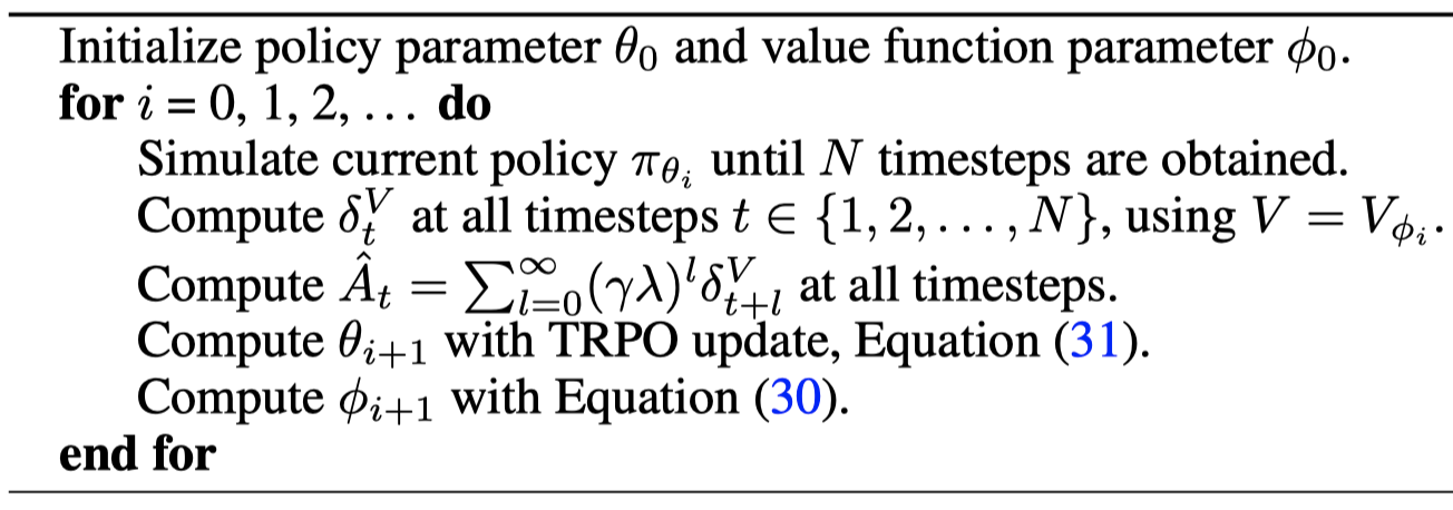
Note that the advantage is computed before the value function update. The authors explain that additional bias would have been introduced if the value function was updated first. In practice, we generally normalize the advantage to have mean zero and standard deviation one to further stablize the process.
Supplementary Materials
Proof
We now prove that Equation \((2)\) is sufficient for Equation \((1)\)
\[\begin{align} \mathbb E_{s_{0:\infty},a_{0:\infty}}\left[\hat A_t(s_{0:\infty}, a_{0:\infty})\nabla_\theta\log\pi_\theta(a_t|s_t)\right]&=\mathbb E_{s_{0:\infty},a_{0:\infty}}\Bigl[\bigl(Q_t(s_{t:\infty}, a_{t:\infty})-b_t(s_{0:t}, a_{0:t-1})\bigr)\nabla_\theta\log\pi_\theta(a_t|s_t)\Bigr]\\\ &=\mathbb E_{s_{0:\infty},a_{0:\infty}}\left[Q_t(s_{t:\infty}, a_{t:\infty})\nabla_\theta\log\pi_\theta(a_t|s_t)\right]\\\ &\quad\quad -\mathbb E_{s_{0:\infty},a_{0:\infty}}\left[b_t(s_{0:t}, a_{0:t-1})\nabla_\theta\log\pi_\theta(a_t|s_t)\right] \end{align}\]Taking a closer look at the first term, we have
\[\begin{align} \mathbb E_{s_{0:\infty},a_{0:\infty}}\Bigl[Q_t(s_{t:\infty}, a_{t:\infty})\nabla_\theta\log\pi_\theta(a_t|s_t)\Bigr] &=\mathbb E_{s_{0:t},a_{0:t}}\Bigl[\mathbb E_{s_{t+1:\infty},a_{t+1:\infty}}[Q_t(s_{t:\infty}, a_{t:\infty})\nabla_\theta\log\pi_\theta(a_t|s_t)]\Bigr]\\\ &=\mathbb E_{s_{0:t},a_{0:t}}\Bigl[\mathbb E_{s_{t+1:\infty},a_{t+1:\infty}}[Q_t(s_{t:\infty}, a_{t:\infty})]\nabla_\theta\log\pi_\theta(a_t|s_t)\Bigr]\\\ &=\mathbb E_{s_{0:t},a_{0:t}}[Q^{\pi,\gamma}(s_{t}, a_{t})\nabla_\theta\log\pi_\theta(a_t|s_t)] \end{align}\]where the last step is obtained because \(E_{s_{t+1:\infty},a_{t+1:\infty}}[Q_t(s_{t:\infty}, a_{t:\infty})] \) is an unbiased estimator of the discounted \( Q \)-function. We follow a similar process to analyze the second term
\[\begin{align} \mathbb E_{s_{0:\infty},a_{0:\infty}}\left[b_t(s_{0:t}, a_{0:t-1})\nabla_\theta\log\pi_\theta(a_t|s_t)\right] &=\mathbb E_{s_{0:t},a_{0:t-1}}\bigl[\mathbb E_{s_{t+1:\infty},a_{t:\infty}}[b_t(s_{0:t}, a_{0:t-1})\nabla_\theta\log\pi_\theta(a_t|s_t)]\bigr]\\\ &=\mathbb E_{s_{0:t},a_{0:t-1}}\bigl[b_t(s_{0:t}, a_{0:t-1})\mathbb E_{s_{t+1:\infty},a_{t:\infty}}[\nabla_\theta\log\pi_\theta(a_t|s_t)]\bigr]\\\ &=\mathbb E_{s_{0:t},a_{0:t-1}}\left[b_t(s_{0:t}, a_{0:t-1})\int_{a_t}\nabla_\theta\log\pi_\theta(a_t|s_t)\pi_\theta(a_t|s_t)da_t\right]\\\ &=\mathbb E_{s_{0:t},a_{0:t-1}}\left[b_t(s_{0:t}, a_{0:t-1})\int_{a_t}\nabla_\theta\pi_\theta(a_t|s_t)da_t\right]\\\ &=\mathbb E_{s_{0:t},a_{0:t-1}}\left[b_t(s_{0:t}, a_{0:t-1})\nabla_\theta\int_{a_t}\pi_\theta(a_t|s_t)da_t\right]\\\ &=\mathbb E_{s_{0:t},a_{0:t-1}}\bigl[b_t(s_{0:t}, a_{0:t-1})\nabla_\theta1\bigr]\\\ &=\mathbb E_{s_{0:t},a_{0:t-1}}\bigl[b_t(s_{0:t}, a_{0:t-1})0\bigr]\\\ &=0 \end{align}\]Therefore, we have
\[\begin{align} &\mathbb E_{s_{0:\infty},a_{0:\infty}}\left[\hat A_t(s_{0:\infty}, a_{0:\infty})\nabla_\theta\log\pi_\theta(a_t|s_t)\right]\\\ =&\mathbb E_{s_{0:\infty},a_{0:\infty}}\left[Q^{\pi,\gamma}(s_t,a_t)\nabla_\theta\log\pi_\theta(a_t|s_t)\right]\\\ =&\mathbb E_{s_{0:\infty},a_{0:\infty}}\left[\big(Q^{\pi, \gamma}(s_t,a_t)-V^{\pi, \gamma}(s_t,)\big) \nabla_\theta\log\pi_\theta(a_t|s_t)\right]\\\ =&\mathbb E_{s_{0:\infty},a_{0:\infty}}\left[A^{\pi, \gamma}(s_t,a_t)\nabla_\theta\log\pi_\theta(a_t|s_t)\right] \end{align}\]where the penultimate step is obtained because \(V^{\pi,\gamma}(s_t)\) does not depends on \(a_t\) and \(\mathbb E_{s_{0:\infty},a_{0:\infty}}[V^{\pi, \gamma}(s_t,)\nabla_\theta\log\pi_\theta(a_t\vert s_t)]=0\). Now that we have derive Equation \((1)\) from the Equation \((2)\), the proof completes.
References
John Schulman et al. High-Dimensional Continuous Control Using Generalized Advantage Estimation