
Importance Weighted Actor-Learner Architecture
IMPALA is a distributed architecture that aims to maximize resource utilization and scale to thousands of machines without sacrificing training stability and data efficiency. It uses the similar architecture as Ape-X with two differences: 1) There is no replay buffer to reuse experiences(although there could be one, which we will discuss later on). 2) It employs a policy-gradient algorithm.
However, the fact that actors and learners work in parallel would result in a policy-lag between the actors and learner — That is, the learner policy \(\pi\) is potentially several updates ahead of the actor’s policy \(\mu\) at the time of update. Extra care must to be taken in order to make the policy-gradient method work in an off-policy fashion. The authors introduce the V-trace off-policy actor-critic algorithm to correct for this hamful discrepancy. In the rest of this section, we first present the overall architecture of IMPALA, and then discuss the V-trace off-policy actor-critic algorithm in details.
Architecture
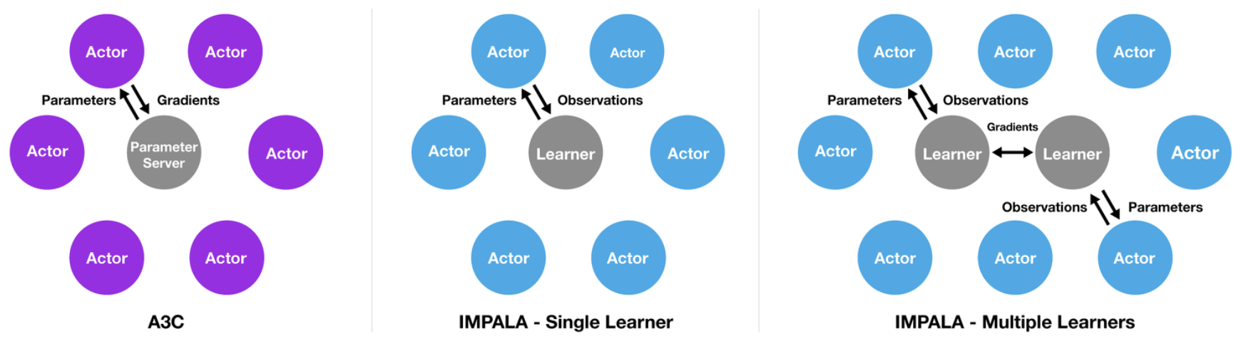
At the beginning of each trajectory, an actor updates its own local policy \(\mu\) to the latest learner policy \(\pi\) and runs it for \(n\) steps in its environment. After \(n\) steps the actor sends the trajectory together with the corresponding policy distributions \(\mu(a_t\vert x_t)\) and initial LSTM state to the learner through a queue. The learner then continuously updates its policy \(\pi\) on batches of trajectories, each collected from many actors. This simple architecture enables the learner(s) to be accelerated using multiple GPUs via parallelism. For example, a learner can apply a convolutional network to all inputs in parallel by folding the time dimension into the batch dimension. Similarly, it can also apply the output layer to all time steps in parallel once all LSTM states are computed.
V-Trace Actor-Critic Algorithm
V-Trace
As in vanilla actor-critic algorithm, we have two networks: the policy network \(\pi_\theta\) and the value function network \(V_\psi\). However, since the policy is updated at the same time actors collect experience, some extra care must be taken to compensate for the policy-lag between the actors and learners. The authors defines the \(n\)-steps V-trace target \(v(x_t)\) for the value function \(V_\psi(s)\) as
\[\begin{align} v(x_t) &:= V(x_t)+\sum_{k=t}^{t+n-1}\gamma^{k-t}\left(\prod_{i=t}^{k-1}c_i\right)\delta_kV\tag {1}\\\ where\quad \delta_kV&:=\rho_k(r_k+\gamma V(x_{k+1})-V(x_k))\\\ c_{i}&:=\lambda \min\left(\bar c, {\pi(a_i|x_i)\over \mu(a_i|x_i)}\right)\\\ \rho_k&:=\min\left(\bar\rho, {\pi(a_k|x_k)\over \mu(a_k|x_k)}\right) \end{align}\]In the above definition, the truncation levels \(\bar c\) and \(\bar\rho\) are hyperparameters and \(\bar\rho\ge\bar c\)(in their experiments, both are set to \(1\)). This truncates the likelihood ratio when \(\pi(a\vert s)\) exceeds \(\mu(a\vert s)\), presenting a conservative update of value function. \(\lambda\) is a discount factor that controls the bias-variance trade-off by exponentially discounting the future error.
Notice that in the on-policy case (when \(\pi=\mu\)), and assuming \(\bar\rho\ge\bar c\ge1\), Equation \((1)\) is reduced to the \(n\)-steps Bellman target
\[\begin{align} v(x_t)&=V(x_t)+\sum_{k=t}^{t+n-1}\gamma^{k-t}\delta_kV\\\ &=\sum_{k=t}^{t+n-1}\gamma^{k-t}r_k +\gamma^n V(x_{t+n}) \end{align}\]It is worth stressing that the truncated importance sampling weights \(c_i\) and \(\rho_k\) play different roles(see the proof in Supplementary Materials):
- The weight \(\rho_k\) impacts the fixed point of \(V(x_k)\), thus the policy \(\pi_{\bar\rho}\). For \(\bar\rho=\infty\) (untruncated \(\rho_t\))we get the value function of the target policy \(V^\pi\), whereas for finite \(\bar\rho\), we evaluate a policy in between behavior policy \(\mu\) and target policy \(\pi\): \(\pi_{\bar\rho}(a\vert x)={\min(\bar\rho\mu(a\vert x),\pi(a\vert x))\over{\sum_{b\in A}\min(\bar\rho\mu(b\vert x),\pi(b\vert x))}}\). So the larger \(\bar\rho\) the smaller the bias in off-policy learning. On the other hand, the variance naturally grows with \(\bar\rho\). However, since we do not take the product of those \(\rho_t\) coefficients, the variance does not explode with the time horizon.
- \(\bar c\) impacts the contraction modulus \(\eta\) of \(\mathcal R\), thus the speed at which V-trace will converge to its fixed point. Intuitively, \(c_t, c_{t+1}, \dots, c_{k-1}\) measures how much a temporal difference \(\delta_kV\) observed at time \(k\) impacts the update of the value function at a previous time \(t\). The more dissimilar \(\pi\) and \(\mu\) are, the larger the variance of this product. We use the truncation level \(\bar c\) as a variance reduction technique. It is important to notice that this truncation does not impact the solution to which the algorithm converges (which is characterized by \(\bar\rho\) only). Moreover, since \(c\) is the ratio of \(\pi\) and \(\mu\), its variance is indirectly affected by the \(\bar\rho\) as \(\bar\rho\) controls the point the policy converges to.
Thus, we see that the truncation levels \(\bar c\) and \(\bar\rho\) represent different features of the algorithm: \(\bar\rho\) impacts the nature of the value function we converge to, whereas \(\bar c\) impacts the speed at which we converge to this function. That’s why we said \(\bar\rho\ge\bar c\). An strange observation from Schmitt et al. 2019 is that increasing \(\bar\rho\) does not provide any performance gain in practice – it even hurts the performance when \(\bar\rho=4\).
Interesting Properties of V-Trace
We can compute the V-trace target recursively as follows:
\[\begin{align} v(x_t)=V(x_t)+\delta_tV+\gamma c_t(v_{t+1}-V(x_{t+1})) \end{align}\]We can consider an additional discounting parameter \(\lambda\in[0,1]\) in the definition of V-trace by multiplying \(c_i\) by \(\lambda\). In the on-policy case, when \(n=\infty\), V-trace then reduces to TD(\(\lambda\)):
\[\begin{align} v(x_t)-V(x_t)&=\sum_{k=t}^\infty(\gamma\lambda)^{k-t}\delta_{k}V\\\ \end{align}\]Actor-Critic Algorithm
Now that we have the target value, we define the corresponding actor and critic losses.
The value loss is just the MSE between the value function and the target
\[\begin{align} \mathcal L(\psi)=\mathbb E_\mu[(v(x_t)-V_\psi(x_t))^2]\tag 2 \end{align}\]The policy loss are the off-policy version of the policy loss in A3C:
\[\begin{align} \mathcal L(\theta)=-\mathbb E_{(x_t,a_t,x_{t+1})\sim\mu}[\rho_t(r_t+\gamma v(x_{t+1})-V_\psi(x_t))\log\pi_\theta(a_t|x_t)]-\mathcal H(\pi_\theta)\tag 3 \end{align}\]where the first term is the vanilla policy gradient loss corrected by importance sampling weights \(\rho_t\) and the second the entropy bonus. Notice that in the advantage term, we use \(v(x_{t+1})\) instead of \(V(x_{t+1})\) to compute the \(Q\) value since the former is the target of the latter, which makes it a better estimate in the context. The authors also experiments on both cases, finding that the \(v(x_{t+1})\) is constantly superior \(V(x_{t+1})\).
Replay Buffer
There could be one replay buffer since the algorithm is off-policy anyway and the authors experiment with replay also finding some improvement on using replay. This is a little confusing to me since the policy-lag experiments show that as the policy-lag increases, performance drops down. Also, as the IMPALA is designed to scale to thousands machine, it may be futile to use a replay since there are always enough new experiences available
Population Based Training
For Population Based Training we use a “burn-in” period of 20 million frames where no evolution is done. This is to stabilize the process and to avoid very rapid initial adaptation which hinders diversity. After collecting 5000 episode rewards in total, the mean capped human normalized score is calculated and a random instance in the population is selected. If the score of the selected instance is more than an absolute \(5\%\) higher, then the selected instance weights and parameters are copied.
No matter if a copy happened or not, each parameter (RMSProp epsilon, learning rate and entropy cost) is permuted with \(33\%\) probability by multiplying with either \(1.2\) or \(1/1.2\).
Discussion
In addition to policy lag, I personally think there is an initial LSTM state lag. One may conteract this undesirable lag by having the worker send its experience to the learner only after a trajectory is done, which enables the agent to recompute the hidden states of LSTMs. However, this may not be desirable for long trajectories.
References
Espeholt, Lasse, Hubert Soyer, Remi Munos, Karen Simonyan, Volodymyr Mnih, Tom Ward, Boron Yotam, et al. 2018. “IMPALA: Scalable Distributed Deep-RL with Importance Weighted Actor-Learner Architectures.” 35th International Conference on Machine Learning, ICML 2018 4: 2263–84.
Schmitt, Simon, Matteo Hessel, and Karen Simonyan. 2019. “Off-Policy Actor-Critic with Shared Experience Replay,” no. Figure 2: 1–20.
Supplementary Materials
Analysis of V-trace
Denote Equation \((1)\) as the V-trace operator \(\mathcal R\):
\[\begin{align} \mathcal RV(x_t) :=& V(x_t)+\mathbb E_\mu\left[\sum_{k\ge t}\gamma^{k-t}\left(\prod_{i=t}^{k-1}c_i\right)\delta_kV\right]\tag 4\\\ where\quad \delta_kV=&\rho_k(r_k+\gamma V(x_{k+1})-V(x_k)) \end{align}\]where the expectation \(\mathbb E_\mu\) is with respect to the behavior policy \(\mu\). Here we consider the infinite horizon operator but very similar results hold for the n-step truncated operator.
Theorem 1. Let \(c_{i}=\lambda \min\left(\bar c, {\pi(a_i\vert x_i)\over \mu(a_i\vert x_i)}\right)\) and \(\rho_k:=\min\left(\bar\rho, {\pi(a_k\vert x_k)\over \mu(a_k\vert x_k)}\right)\) be the truncated importance sampling weights, with \(\bar\rho\ge \bar c\). Assume that there exists \(\beta\in(0,1]\) such that \(\mathbb E_\mu\rho_0\ge\beta\). Then the operator \(\mathcal R\) has a unique fixed point \(V^{\pi_{\bar\rho}}\), which is the value function of the policy \(\pi_{\bar\rho}\) defined by
\[\begin{align} \pi_{\bar\rho}(a|x)={\min(\bar\rho\mu(a|x),\pi(a|x))\over{\sum_{b\in A}\min(\bar\rho\mu(b|x),\pi(b|x))}}\tag 5 \end{align}\]Furthermore, \(\mathcal R\) is a \(\eta\)-contraction mapping in sup-norm with
\[\begin{align} \eta:=\gamma^{-1}-(\gamma^{-1}-1)\mathbb E_\mu\left[\sum_{t\ge0}\gamma^t\left(\prod_{i=0}^{t-2}c_i\right)\rho_{t-1}\right]\le 1-(1-\gamma)\beta< 1\tag 6 \end{align}\]Before we prove Theorem 1, let’s see the role of \(\bar c\) and \(\bar \rho\) play. \(\bar c\) appearing the contraction modulus \(\eta\) affects the speed at which V-trace converges to \(V^{\pi_\bar\rho}\) – a small \(\bar c\) corresponds to lower variance but worse contraction rate. On the other hand, \(\bar\rho\) influences the policy \(\pi_{\bar\rho}\) and thus controls the fixed point \(V^{\pi_\bar\rho}\). Moreover, \(\bar\rho\) biases the policy and thus the value function whenever \(\bar\rho\mu(a\vert x)<\pi(a\vert x)\), which makes the V-Trace operator inappropriate for data way off policy.
Proof. First notice that we can rewrite Equation \((2)\) as
\[\begin{align} \mathcal R V(x_t)=(1-\mathbb E_\mu\rho_t)V(x_t)+\mathbb E_\mu\left[\sum_{k\ge t}\gamma^{k-t}\left(\prod_{i=t}^{k-1}c_i\right)\big(\rho_kr_k+\gamma(\rho_k-c_k\rho_{k+1})V(x_{k+1})\big)\right] \end{align}\]where we move \(-\rho_{k+1}V(x_{k+1})\) in \(\delta_{k+1}V\) into \(\delta_{k}V\). Therefore, we have
\[\begin{align} \mathcal RV_1(x_{t})-\mathcal RV_2(x_t)&=(1-\mathbb E_\mu\rho_t)(V_1(x_t)-V_2(x_t))+\mathbb E_\mu\left[\sum_{k\ge t}\gamma^{k-t+1}\left(\prod_{i=t}^{k-1}c_i\right)\big((\rho_k-c_k\rho_{k+1})(V_1(x_{k+1})-V_2(x_{k+1})\big)\right]\\\ &=\mathbb E_\mu\left[\sum_{k\ge t}\gamma^{k-t}\left(\prod_{i=t}^{k-2}c_i\right)\big(\underbrace{(\rho_{k-1}-c_{k-1}\rho_{k})}_{\alpha_k}(V_1(x_{k})-V_2(x_{k})\big)\right] \end{align}\]with the notation that \(c_{t-1}=\rho_{t-1}=1\) and \(\prod_{i=t}^{k-2}c_i=1\) for \(k=t\) and \(t+1\).
We shall see the coefficients \((\alpha_k)_{k\ge t}\) are non-negative in expectation. Because \(\bar\rho\ge \bar c\), we have
\[\begin{align} \mathbb E_\mu\alpha_k=\mathbb E_\mu[\rho_{k-1}-c_{k-1}\rho_k]\ge\mathbb E_\mu[c_{k-1}(1-\rho_k)]\ge 0 \end{align}\]since \(\mathbb E_\mu\rho_k\le\mathbb E_\mu\log{\pi(a_k\vert x_k)\over\mu(a_k\vert x_k)}=1\). Thus \(V_1(x_{t})-V_2(x_t)\) is a linear combination of the values \(V_1-V_2\) at other states, weighted by non-negative coefficients whose sum is
\[\begin{align} &\sum_{k\ge t}\gamma^{k-t}\mathbb E_\mu\left[\left(\prod_{i=t}^{k-2}c_i\right)(\rho_{k-1}-c_{k-1}\rho_{k})\right]\\\ =&\sum_{k\ge t}\gamma^{k-t}\mathbb E_\mu\left[\left(\prod_{i=t}^{k-2}c_i\right)\rho_{k-1}\right]-\sum_{k\ge t}\gamma^{k-t}\mathbb E_\mu\left[\left(\prod_{i=t}^{k-1}c_i\right)\rho_{k}\right]\\\ &\qquad\color{red}{\text{add }\gamma^{-1}(\mathbb E_{\mu}\rho_{t-1}-1)\text{ to the second term and rearange}}\\\ =&\sum_{k\ge t}\gamma^{k-t}\mathbb E_\mu\left[\left(\prod_{i=t}^{k-2}c_i\right)\rho_{k-1}\right]-\gamma^{-1}\left(\sum_{k\ge t}\gamma^{k-t}\mathbb E_\mu\left[\left(\prod_{i=t}^{k-2}c_i\right)\rho_{k-1}\right]-1\right)\\\ =&\gamma^{-1}-(\gamma^{-1}-1)\sum_{k\ge t}{\gamma^{k-t}\mathbb E_\mu\left[\left(\prod_{i=t}^{k-2}c_i\right)\rho_{k-1}\right]}=\eta\\\ &\qquad\color{red}{\sum_{k\ge t}{\gamma^{k-t}\mathbb E_\mu\left[\left(\prod_{i=t}^{k-2}c_i\right)\rho_{k-1}\right]}\ge\sum_{k=t}^{t+1}{\gamma^{k-t}\mathbb E_\mu\left[\left(\prod_{i=t}^{k-2}c_i\right)\rho_{k-1}\right]}=1+\gamma\mathbb E_\mu\rho_t}\\\ &\qquad\color{red}{\gamma<1\text{ and }(\gamma^{-1}-1)>0}\\\ \le&\gamma^{-1}-(\gamma^{-1}-1)(1+\gamma\mathbb E_\mu\rho_t)\\\ =& 1-(1-\gamma)\mathbb E_\mu\rho_t\\\ &\qquad\color{red}{\mathbb E_\mu\rho_t\ge\beta}\\\ \le& 1-(1-\gamma)\beta\\\ &\qquad\color{red}{\beta\in(0, 1]}\\\ \le&\gamma<1 \end{align}\]We deduce that \(\Vert\mathcal RV_1(x_t)-\mathcal RV_1(x_t)\Vert\le \eta\Vert V_1-V_2\Vert_\infty\), with \(\eta\) defined in Equation \((4)\), so \(\mathcal R\) is a contraction mapping. Thus \(\mathcal R\) possesses a unique fixed point. Let us now prove that this fixed point is \(V^{\pi_\bar\rho}\). We have
\[\begin{align} &\mathbb E_\mu[\rho_t(r_t+\gamma V^{\pi_\bar\rho}(x_{t+1})-V^{\pi_\bar\rho}(x_t))|x_t]\\\ =&\sum_a\mu(a|x_t)\min\left(\bar\rho, {\pi(a|x_t)\over \mu(a|x_t)}\right)\left(r_t+\gamma\sum_{x_{t+1}} p(x_{t+1}|x_t,a)V^{\pi_\bar\rho}(x_{t+1})-V^{\pi_\bar\rho}(x_t)\right)\\\ =&\sum_a\left(r_t+\gamma\sum_{x_{t+1}} p(x_{t+1}|x_t,a)V^{\pi_\bar\rho}(x_{t+1})-V^{\pi_\bar\rho}(x_t)\right)\min\left(\bar\rho\mu(a|x_t), {\pi(a|x_t)}\right)\\\ =&\underbrace{\sum_a\pi_{\bar\rho}(a|x_t)\left(r_t+\gamma\sum_{x_{t+1}} p(x_{t+1}|x_t,a)V^{\pi_\bar\rho}(x_{t+1})-V^{\pi_\bar\rho}(x_t)\right)}_{=0,\text{ since }V^{\pi_\bar\rho}\text{ is the value function of }{\pi_\bar\rho}}\sum_{b\in A}\min(\bar\rho\mu(b|x_t),\pi(b|x_t))\\\ =&0 \end{align}\]Therefore \(\delta_kV^{\pi_\bar\rho}=0\) and \(\mathcal RV^{\pi_\bar\rho}=V^{\pi_\bar\rho}\), i.e, \(V^{\pi_\bar\rho}\) is the unique fixed point of \(\mathcal R\).