
Introduction
In this post, we present a model-based meta-RL framework that can adapt fast to changes of environment dynamics. Long story short, this method learns a dynamics model that can fast adapt to the environment changes and uses this model to do model predictive control(MPC) to take actions. It is worth noting that the adaptive nature of the learned model is especially important not only in meta-learning but also in model-based RL since it alleviates the requirement of a globally accurate model, which plays an important role in model-based RL.
TL; DR
MB-MRL learns an adaptive dynamics model parameterized by \(\theta\) such that we can update it to obtain a desired dynamics model \(\theta’=u_\psi(\tau(t-M, t-1);\theta)\) according to the past \(M\) steps. With the updated dynamics model \(\theta’\), the agent use an MPC method to select an action.
Learning an adaptive dynamics model with parameters \(\theta\) can be done by meta-learning. In particular, when we use MAML, this boils down to the following optimization problem
\[\begin{align} \min_{\theta,\psi}\mathbb E_{\tau(t,t+K)\sim\mathcal D}[&\mathcal L(\tau(t,t+k),\theta')]\\\ s.t.\quad \theta'=u_\psi(\tau(t-M,t-1);\theta)=&\theta-\psi\nabla_\theta\mathcal L(\tau(t-M,t-1);\theta)\\\ \end{align}\]where the predictive loss \(\mathcal L(\theta)={1\over M}\sum_{i=t-M}^{t-1}((s_{i+1}-s_i)-f(s_i,a_i);\theta)\) minimizes the prediction of the change in consecutive states.
Preliminaries
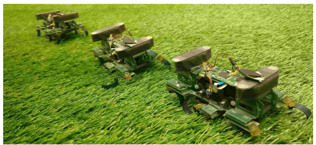
We define a distribution of environment \(\mathcal E\) as \(\rho(\mathcal E)\). We forgo the episodic framework, where tasks are pre-defined to be different rewards or environments, and tasks exists at the trajectory level only. Instead, we consider each timestep to potentially be a new “tasks”, where any detail or setting could have changed at any timestep. For example, a real legged millirobot unexpectedly loses a leg when moving forward as the following figure shows
We assume that the environment is locally consistent, in that every segment of length \(j-i\) belongs to same environment. Even though this assumption is not always correct, it allows us to learn to adapt from data without knowing when the environment has changed. Due to the fast nature of adaptation (less than a second), this assumption is seldom violated.
Problem Setting
We formulate the adaptation problem as an optimization problem for the parameters of learning procedure \(\theta,\psi\) as follows:
\[\begin{align} \min_{\theta,\psi}\mathbb E_{\mathcal E\sim\rho(\mathcal E)}\big[\mathbb E_{\tau_{\mathcal E}(t-M,t+K)\sim\mathcal D}[\mathcal L(\tau_{\mathcal E}(t,t+K), \theta'_{\mathcal E})]\big]\tag {1}\\\ s.t. \theta'_{\mathcal E}=u_\psi(\tau_{\mathcal E}(t-M, t-1), \theta) \end{align}\]where \(\tau_{\mathcal E}(\cdot,\cdot)\) corresponds to trajectory segments sampled from previous experiences, \(u_\psi\) is the adaptation process, which updates the dynamics model with parameters \(\theta\) using the past \(M\) data points. \(\mathcal L\) denotes the dynamics loss function, which, as we discussed in the previous post, is the mean squared error of changes in state \(\Delta s\)(see the official implementation here):
\[\begin{align} \mathcal L(\tau_{\mathcal E}(t,t+K),\theta'_{\mathcal E})={1\over K}\sum_{k=t}^{t+K-1}\big((s_{k+1} - s_{k})-f_{\theta}(s_{k},a_{k})\big)^2 \end{align}\]Intuitively, by optimizing Eq.\((1)\), we expect to learn an adaptive dynamics model with parameters \(\theta\), with which the agent is able to adapt the model to \(\theta’_{\mathcal E}\) according to the past \(M\) transitions.
Also, notice that in Eq.\((1)\), we put all data in a single dataset \(\mathcal D\) instead of maintaining one dataset for each task since we want to do fast adaptation instead of task transfer here.
Benefit of Combining Meta-Learning with Model-Based RL
Learning to adapt a model alleviates a central challenge of model-based reinforcement learning: the problem of acquiring a global model that is accurate throughout the entire state space. Furthermore, even if it were practical to train a globally accurate dynamics model, the dynamics inherently change as a function of uncontrollable and often unobservable environmental factors. If we have a model that can adapt online, it need not be perfect everywhere a priori. This property has previously been exploited by adaptive control methods (Åström and Wittenmark, 2013; Sastry and Isidori, 1989; Pastor et al., 2011; Meier et al., 2016); but, scaling such methods to complex tasks and nonlinear systems is exceptionally difficult. Even when working with deep neural networks, which have been used to model complex nonlinear systems (Kurutach et al., 2018), it is exceptionally difficult to enable adaptation, since such models typically require large amounts of data and many gradient steps to learn effectively. By specifically training a neural network model to require only a small amount of experience to adapt, we can enable effective online adaptation in complex environments while putting less pressure on needing a perfect global model. (excepted from the original paper)
Model-Based Meta-Reinforcement Learning
Nagabandi&Clavera et al. introduce two approaches to solve Objective.\((1)\). One is based on gradient-based meta-learning, the other is based on recurrent models. Both share the same framework and only differ in network architecture and optimization procedure. In fact, since they orthogonally emphasize different parts of the framework, they may be combined to form a more powerful method in the end.
Gradient-Based Adaptive Learner
Gradient-Based Adaptive Learner(GrBAL) uses a gradient-based meta-learning to perform online adaptation; in particular, we use MAML. In this case, the update rule is prescribed by gradient descent:
\[\begin{align} \theta'_{\mathcal E}=u_\psi(\tau_{\mathcal E}(t-M, t-1), \theta)=\theta_{\mathcal E}+\psi\nabla_{\theta}{1\over M}\sum_{m=t-M}^{t-1}\big((s_{m+1} - s_{m})-f_{\theta}(s_{m},a_{m})\big)^2 \end{align}\]Here \(\psi\) is the step sizes at adaptation time.
Recurrence-Based Adaptive Learner
Recurrence-Based Adaptive Learner(ReBAL) utilizes a recurrent model(or attention model), which learns its own update rule through its internal structure. In this case, \(\psi\) and \(u_\psi\) correspond to the weights of the recurrent model.
Algorithm
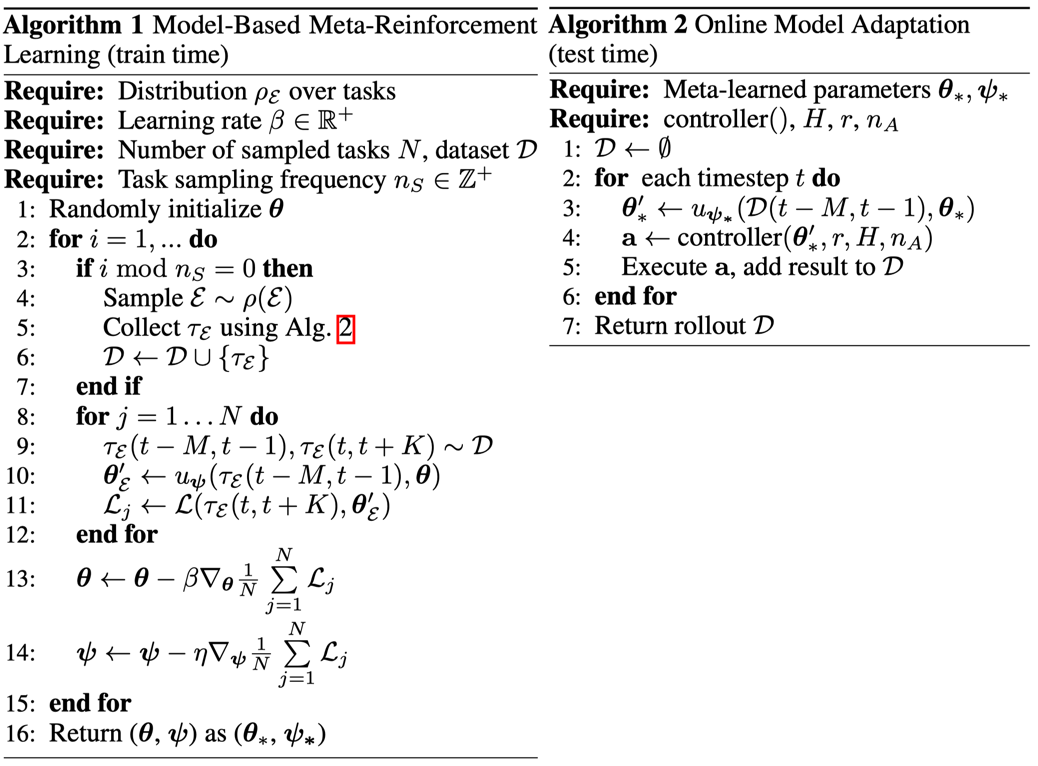
If you’ve already familiar with model-agnostic meta-learning and model predictive control(MPC), there is nothing new here. We learn an adaptive dynamics model via Algorithm 1, and then at each time step, the agent first adapts the model and then perform MPC to select actions as shown in Algorithm 2. The planning horizon \(H\) is smaller than the adaptation horizon \(K\) since the adapted model is only valid within the current context.
Experimental Results
See the following video for experimental results
References
Anusha Nagabandi, Ignasi Clavera, Simin Liu, Ronald S. Fearing, Pieter Abbeel, Sergey Levine, & Chelsea Finn, “Learning to Adapt in Dynamic, Real-World Environments through Meta-Reinforcement Learning,” ICLR, pp. 1–17, 2019.
C. Finn, P. Abbeel, and S. Levine, “Model-agnostic meta-learning for fast adaptation of deep networks,” 34th Int. Conf. Mach. Learn. ICML 2017, vol. 3, pp. 1856–1868, 2017.
Y. Duan, J. Schulman, X. Chen, P. L. Bartlett, I. Sutskever, and P. Abbeel, “RL\(^2\): Fast Reinforcement Learning via Slow Reinforcement Learning,” ICLR, pp. 1–14, 2017.