
Introduction
Self-Attention Generative Adversarial Networks(SAGAN), a structure proposed by Han Zhang et al. in PMLR 2019, has experimentally shown to significantly outperform prior work in image synthesis. In this post, we discuss several techniques involved in SAGAN, including self-attention, spectral normalization, conditional batch normalization, projection discriminator, etc.
Bonus: we will give simple exemplary code for each key components, but you should be aware that the code provided here is simplified only for illustrative purpose. For the whole practical implementation, you may refer to my repo for SAGAN on GitHub, or the official implementation from Google Brain.
Self-Attention
Motivation
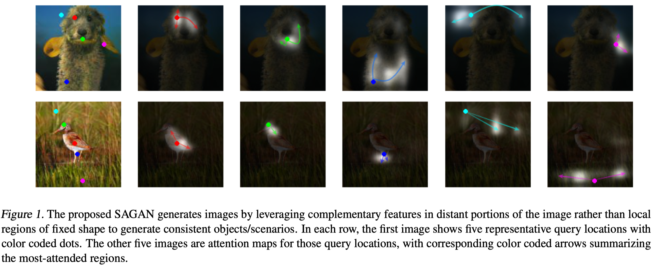
GANs has shown their success in modeling structural texture, but they often fail to capture geometric or structural patterns that occur consistently in some classes. For example, synthesized dogs are often drawn with realistic fur texture but without clearly defined separate feet. One explanation for this is that convolutional layers are good at capturing local structures, but they have trouble discovering long-range dependencies: 1). Although deep ConvNets are theoretically capable of capturing long-range dependencies, it is hard for optimization algorithms to find parameter values that carefully coordinate multiple layers to capture these dependencies, and these parameters may be statistically brittle and prone to failure when applied to previously unseen data. 2). Large convolutional kernels increase the representational capacity but are more computationally inefficient.
Self-attention, on the other hand, exhibits a better balance between the ability to model long-range dependencies and computational and statistical efficiency. Based on these ideas, Han Zhang et al. proposed SAGANs to introduce a self-attention mechanism into convolutional GANs.
Self-Attention with Images
We have discussed the self-attention mechanism in the previous post, which is applied to 3D sequential data to capture temporal dependencies. To apply self-attention to images, Han Zhang et al. suggest to make three major modifications:
-
Replace fully connected layers with 1-by-1 convolutional layers.
-
Reshape 4D tensors into 3D tensors(merging height and width together) before computing attention and reshape them back afterward.
-
Multiply the output of the attention layer by a scale parameter and add it back to the input feature map:
where o is the output of the attention layer and \(\gamma\) is a learnable scalar initialized to 0. Introducing the learnable \(\gamma\) allows the network to first rely on the cues in the local neighborhood — since this is easier — and then gradually learn to assign more weight to the non-local evidence. The intuition for why we do this is straightforward: we want to learn the easy task first and then progressively increase the complexity of the task. [1]
Python Code
def attention(q, k, v):
  # softmax(QK^T)V
  # we do not rescale the dot-product as in Transformer
  # since the dimension is generally small and saturation may not happen
  dot_product = tf.matmul(q, k, transpose_b=True) # [B, H, N, N]
  weights = tf.nn.softmax(dot_product)            # [B, H, N, V]
  x = tf.matmul(weights, v)

  return x

def conv_attention(x, key_size=None, name="ConvAttention"):
  """ attention based on SA-GAN
 	The official implementation downsamples g and h via maxpooling layer
 	but we do not do it here for simplicity
  """
  H, W, C = x.shape.as_list()[1:]
  if key_size is None:
    key_size = C // 8   # default implementation suggested by SAGANs
  with tf.variable_scope(name):
    # conv is either a plain convolution or a spectral normalized convolution
    # whose arguments are (input, filters, kernel_size, stride, name=None)
    f = conv(x, key_size, 1, 1, name="f")
    g = conv(x, key_size, 1, 1, name="g")
    h = conv(x, C, 1, 1, name="h")

    f = tf.reshape(f, [-1, H * W, key_size])
    g = tf.reshape(g, [-1, H * W, key_size])
    h = tf.reshape(h, [-1, H * W, C])

    o = attention(f, g, h)
    o = tf.reshape(o, [-1, H, W, C])
    o = conv(o, C, 1, 1)

    gamma = tf.get_variable('gamma', [1], initializer=tf.zeros_initializer())
    x = gamma * o + x		# residual connection

  return x
Spectral Normalization
Motivation
Before getting into the details of spectral normalization, we briefly introduce some basic ideas to ensure we are on the same page.
- A flat local minimum of a function is less sensitive to the input perturbation(see figure bellow for illustration).
- A Hessian matrix describes the local curvature of a multi-variate function; it measures the sensitivity of a function to its input at a local minimum.
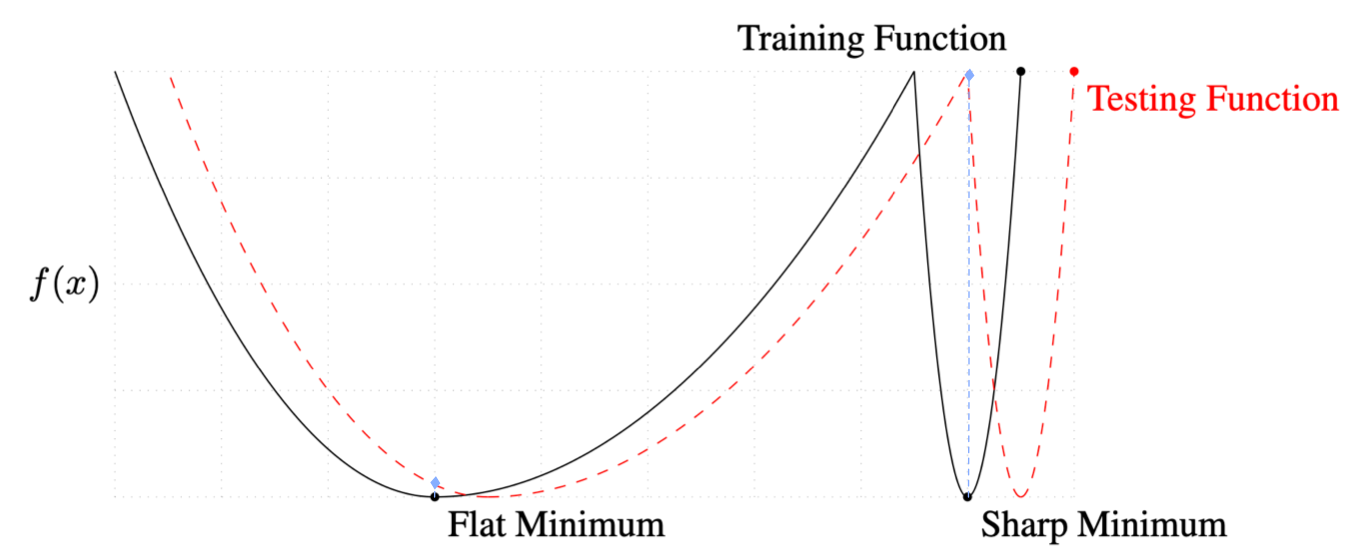
Yuichi Yoshida et al.[3] stress that a flat local minimum of a loss function generalizes better than a sharp one(according to (1)), and they formulate the flatness as the eigenvalues of the Hessian matrix of the loss function(according to (2)). Following this thought, they prove that, if all activation functions are piecewise linear(e.g. ReLU), to achieve a flat local minimum, it is sufficient to bound the spectral norm of the weight matrix at each layer. Therefore, they propose to regularize the spectral norm of each weight matrix in the loss function just like L2 regularization.
Based on Y. Yoshida’s work, Takeru Miyato et al. in [2] develope spectral normalization, which explicitly normalizes the spectral norm of the weight matrix in each layer so that it satisfies the Lipschitz constraints \(\sigma(W)=1\):
\[\begin{align} W_{SN}(W):=W/\sigma(W) \end{align}\]where \(\sigma(W)\) is the spectral norm of \(W\). We can verify its spectral norm by showing
\[\begin{align} \sigma(W_{SN}(W))=\sigma(W)/\sigma(W)=1 \end{align}\]Takeru Miyato et al. further prove that spectral normalization regularizes the gradient of \(W\), preventing the column space of \(W\) from concentrating into one particular direction. This precludes the transformation of each layer from becoming sensitive in one direction.
How to Compute The Spectral Norm?
Assume \(W\) is of shape \((N, M)\) and we have a randomly initialized vector \(u\). The power iteration method computes the spectral norm of \(W\) as follows
\[\begin{align} &\mathbf{For}\ i= 1...T:\\\ &\quad v = W^Tu/\Vert W^Tu\Vert_2\\\ &\quad u = Wv/\Vert Wv\Vert_2\\\ &\sigma(W)=u^TWv \end{align}\]where \(u\) and \(v\) approximate the first left and right singular vector of \(W\). In practice, \(T=1\) is sufficient since we gradually update \(W\) as well.
Python Code
def spectral_norm(w, iteration=1):
  w_shape = w.shape.as_list()
  w = tf.reshape(w, [-1, w_shape[-1]])    # [N, M]

  # [1, M]
  u_var = tf.get_variable('u', [1, w_shape[-1]],
                          initializer=tf.truncated_normal_initializer(),
                          trainable=False)
  u = u_var
	# power iteration
  for _ in range(iteration):
    v = tf.nn.l2_normalize(tf.matmul(u, w, transpose_b=True))   # [1, N]
    u = tf.nn.l2_normalize(tf.matmul(v, w))                     # [1, M]

  sigma = tf.squeeze(tf.matmul(tf.matmul(v, w), u, transpose_b=True))   # scalar
  w = w / sigma

  with tf.control_dependencies([u_var.assign(u)]):	# we reuse the value of u
    w = tf.reshape(w, w_shape)

  return w

def snconv(x, filters, kernel_size, strides=1, padding='SAME', name="snconv"):
  """ Spectral normalized convolutional layer """
  H = W = kernel_size

  with tf.variable_scope(name):
    w = tf.get_variable('weight', shape=[H, W, x.shape[-1], filters],
                        initializer=tf.contrib.layers.xavier_initializer())
    w = spectral_norm(w)
    x = tf.nn.conv2d(x, w, strides=(1, strides, strides, 1), padding=padding)

    b = tf.get_variable('bias', [filters], initializer=tf.zeros_initializer())
    x = tf.nn.bias_add(x, b)

  return x
Conditional Batch Normalization
The conditional batch normalization was first proposed by Harm de Vries, Florian Strub et al. [4]. The central idea is to condition the \(\gamma\) and \(\beta\) of the batch normalization on some \(x\)(e.g., language embedding), which is done by adding \(f(x)\) and \(h(x)\) to \(\gamma\) and \(\beta\), respectively. Here, \(f\) and \(h\) could be any function(e.g. a one-hidden-layer MLP). In this way, they are able to incorporate some additional information into a pre-trained network with minimal overhead.
SAGAN could be implemented as a form of conditional GANs(cGANs) by integrating class labels into both the generator and discriminator. In the generator, this is achieved through conditional batch normalization layers, where we give each label a specific gamma and beta. In the discriminator, this is accomplished by projection, a method we will see soon in the next section. Here we provide the code for conditional batch normalization from [7] with some annotations.
class ConditionalBatchNorm:
  """Conditional BatchNorm.
  For each class, it has a specific gamma and beta as normalization variable.
  """
  def __init__(self, num_categories, name="conditional_batch_norm", decay_rate=0.999):
    with tf.variable_scope(name):
      self.name = name
      self.num_categories = num_categories
      self.decay_rate = decay_rate

  def __call__(self, inputs, labels, is_training=True):
    # denote number of classes as N, number of features(channels) as F, length of labels as L
    inputs = tf.convert_to_tensor(inputs)
    inputs_shape = inputs.get_shape()
    params_shape = inputs_shape[-1:]  # F
    axis = [0, 1, 2]
    shape = tf.TensorShape([self.num_categories]).concatenate(params_shape) # [N, F]
    moving_shape = tf.TensorShape([1, 1, 1]).concatenate(params_shape)    # [1, 1, 1, F]

    with tf.variable_scope(self.name):
      # [N, F]
      self.gamma = tf.get_variable('gamma', shape,
                                   initializer=tf.ones_initializer())
      # [N, F]
      self.beta = tf.get_variable('beta', shape,
                                  initializer=tf.zeros_initializer())
      # [1, 1, 1, F]
      self.moving_mean = tf.get_variable('mean', moving_shape,
                                         initializer=tf.zeros_initializer(),
                                         trainable=False)
      # [1, 1, 1, F]
      self.moving_var = tf.get_variable('var', moving_shape,
                                        initializer=tf.ones_initializer(),
                                        trainable=False)

      beta = tf.gather(self.beta, labels)   # [L, F]
      beta = tf.expand_dims(tf.expand_dims(beta, 1), 1) # [L, 1, 1, F]
      gamma = tf.gather(self.gamma, labels) # [L, F]
      gamma = tf.expand_dims(tf.expand_dims(gamma, 1), 1) # [L, 1, 1, F]
      decay = self.decay_rate
      variance_epsilon = 1e-5
      if is_training:
        mean, variance = tf.nn.moments(inputs, axis, keep_dims=True)
        update_mean = tf.assign(self.moving_mean, self.moving_mean * decay + mean * (1 - decay))
        update_var = tf.assign(self.moving_var, self.moving_var * decay + variance * (1 - decay))
        tf.add_to_collection(tf.GraphKeys.UPDATE_OPS, update_mean)
        tf.add_to_collection(tf.GraphKeys.UPDATE_OPS, update_var)
        outputs = tf.nn.batch_normalization(
            inputs, mean, variance, beta, gamma, variance_epsilon)
      else:
        outputs = tf.nn.batch_normalization(
              inputs, self.moving_mean, self.moving_var, beta, gamma, variance_epsilon)
      outputs.set_shape(inputs_shape)
      return outputs
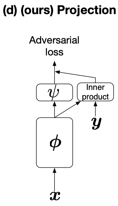
Projection Discriminator
In [5], Takeru Miyato proposes to incorporate class labels into the discriminator. To see how it works, we denote the conditional discriminator as \(D(x,y)=\sigma(f(x,y))\), where the \(f(x,y)\) is a function of \(x\) and \(y\). We first derive the optimal discriminator by setting the derivative of \(D\) to zero
\[\begin{align} &\nabla_D(-\mathbb E_{x,y\sim p_{data}}[\log D(x,y)]-E_{x,y\sim q(x,y)}[\log(1-D(x,y))])\\\ =&\int_{x,y}-p_{data}(x,y){1\over D(x,y)}+q(x,y){1\over 1-D(x,y)}=0 \end{align}\]Solving this equation, we get the optimal discriminator
\[\begin{align} D^\*(x,y)={p_{data}(x,y)\over p_{data}(x,y)+q(x,y)} \end{align}\]By replacing the discriminator with \(\sigma(f(x,y))\), we have
\[\begin{align} {1\over1+\exp(-f(x,y))}&={p_{data}(x,y)\over p_{data}(x,y)+q(x,y)}\\\ \end{align}\]This gives us the logits
\[\begin{align} f(x,y)&=\log{p_{data}(x,y)\over q(x,y)}\\\ &=\log{p_{data}(y|x)\over q(y|x)}+\log {p_{data}(x)\over q(x)}\\\ &=r(y|x)+r(x) \end{align}\]Now we take a closer look at \(p(y\vert x)\), a categorical distribution usually expressed as a softmax function, whose log-linear model is
\[\begin{align} \log p(y=c|x)=v^T\phi(x)+\log Z(\phi(x)) \end{align}\]where \(Z(\phi(x))\) is the partition function. The log-likelihood ratio, therefore, would take the following form:
\[\begin{align} r(y|x)=(v_p-v_q)^T\phi(x)-\big(\log Z_p(\phi(x))-\log Z_q(\phi(x))\big) \end{align}\]Now, define \(v=v_p-v_q\), and put the normalization constant together with \(r(x)\) into one expression \(\psi(\phi(x))\). We can rewrite \(f(x,y)\) as
\[\begin{align} f(x,y=c)=v^T\phi(x)+\psi(\phi(x)) \end{align}\]If we use \(y\) to denote a one-hot vector of the label and use \(V\) to denote the embedding matrix consisting of the row vectors \(v^T\), we can rewrite the above model by
\[\begin{align} f(x,y)=y^TV\phi(x)+\psi(\phi(x)) \end{align}\]This formulation introduces the label information via an inner product as shown in the following figure.
Python Code
def embedding(x, n_classes, embedding_size, name="embedding"):
  with tf.variable_scope(name):
    embedding_map = tf.get_variable(name="embedding_map",
                                    shape=[n_classes, embedding_size],
                                    initializer=tc.layers.xavier_initializer())
    embedding_map_trans = spectral_norm(tf.transpose(embedding_map))
    embedding_map = tf.transpose(embedding_map_trans)

    return tf.nn.embedding_lookup(embedding_map, x)

# x is a 4D tensor from the previous ConvNet: [B, H, W, C]
x = lrelu(x)
x = tf.reduce_sum(x, [1, 2])					# phi(x) 			[B, C]
out = dense(x, 1, name="FinalLayer")	# psi(phi(x)) [B, 1]
# y^TVphi(x)
y = embedding(label, n_classes, C, True)						# y^TV 				[B, C]
y = tf.reduce_mean(x * y, axis=1, keep_dims=True)		# y^TVphi(x)	[B, 1]
out += y		# f(x, y) [B, 1]]
Miscellanea
In this section, we briefly mention several other techniques adopted by SAGANs
- SAGANs use the hinge loss as the adversarial loss, which is defined as
- SAGANs use different learning rate for the generator and discriminator, which is so-called Two-Timescale Update Rule (TTUR). For ImageNet, they use 0.0004 for the discriminator and 0.0001 for the generator. In my implementation, I use 0.0001 for the discriminator and 0.00005 for the generator for celebA.
References
- Han Zhang et al. Self-Attention Generative Adversarial Networks. In ICML 2019.
- Takeru Miyato et al. Spectral Normalization for Generative Adversarial Networks. In ICLR 2018
- Yuichi Yoshida et al. Spectral Norm Regularization for Improving the Generalizability of Deep Learning
- Harm de Vries, Florian Strub et al. Modulating early visual processing by language
- Takeru Miyato, Masanori Koyama. cGANs with Projection Discriminator
- Official Code for SAGAN
- A detailed discussion on spectral norm by Christian Cosgrove