
Introduction
In this post, we will talk about a set of policy gradient mothods. In general, for each algorithm, I’ll give the corresponding pseudocode first, and then explore them in detail — demonstrate the relevant concept, core ideas, and contributions.
This will be a long journey, feel free to grab yourself a coffee first. Hope you’ll enjoy it :-)
Update Note
Maybe I should have discussed stochastic and deterministic policy gradient separately since they in fact belongs to two different categories of learning process: the stochastic ones are on-policy while the deterministic ones are off-policy.
Table of Contents
Policy-Gradient RL
Policy Gradient
Define the policy objective function as maximizing the expected rewards of trajectories, \( J(\theta)=\mathbb E_{p(\tau;\theta)}[r(\tau)]=\int_\tau r(\tau) p(\tau;\theta)d\tau \), where \( \tau \) is a trajectory and \( r(\tau) \) is the total discounted reward along the trajectory
To maximize the policy objective function, we first define \( \Delta\theta \),
\[\begin{align} \Delta \theta=\alpha \nabla_\theta J(\theta) \end{align}\]Then calculate the policy gradient
\[\begin{align} \nabla_\theta J(\theta)&=\int_\tau r(\tau)\nabla_\theta p(\tau;\theta)d\tau\\\ &=\int_\tau \bigl(r(\tau)\nabla_\theta \log p(\tau;\theta)\bigr)p(\tau;\theta)d\tau\\\ &=\mathbb E\left[r(\tau)\nabla_\theta \log p(\tau;\theta)\right] \end{align}\]where the first step is obtained following Leibniz’s integral rule.
We decompose the probability of a trajectory as follows
\[\begin{align} p(\tau;\theta)=p(s_0)\prod_{t\ge0} p(s_{t+1}|s_t, a_t)\pi_\theta (a_t|s_t) \end{align}\]so that the log likelihood becomes
\[\begin{align} \log p(\tau;\theta)=\log p(s_0) + \sum_{t\ge0}\bigl( \log p(s_{t+1}|s_t, a_t)+\log\pi_\theta(a_t|s_t)\bigr) \end{align}\]Then we differentiate it
\[\begin{align} \nabla_\theta\log p(\tau;\theta)=\sum_{t\ge0}\nabla_{\theta} \log\pi_\theta(a_t|s_t) \end{align}\]Note that the above equation does not depend on the transition probability, which suggests the policy gradient algorithm is model-free.
Suming them up, we obtain
\[\begin{align} \nabla_\theta J(\theta)&=\mathbb E\left[ \sum_{t\ge0}r(\tau)\nabla_\theta \log \pi_\theta(a_t|s_t)\right] \end{align} \tag {1}\]which can be approximated using sampled trajectories.
Furthermore, since policy at time step \( t \) should not take effect on the rewards in the past, we reframe the gradient of the objective function so that we can approximate it simply by the cumulative future reward from that state instead of that of the whole trajectory(this is, sometimes, referred to as causality, could be regarded as a variance reduction technique since now the number of reward signals is reduced, and hence, there is much less stochasticity in the reward signals. Mathematically, the variance is diminished thanks to the shrinked range of the advantages.):
\[\begin{align} \nabla_\theta J(\theta)&=\mathbb E\left[ \sum_{t}\left(\sum_{t'\ge t}\gamma^{t'-t}r_{t'}\right)\nabla_\theta \log \pi_\theta(a_t|s_t)\right]\\\ &= \mathbb E\left[Q(s, a)\nabla_\theta \log \pi_\theta(a|s)\right] \end{align}\tag {2}\]where, in the first step, we replace the whole trajectory reward with \( Q(s_t, a_t)=\sum_{t’\ge t}\gamma^{t’-t}r_{t’} \) and, in the second step, we merge the timestamp into the expectation.
\( \nabla_\theta \log\pi_\theta(a\vert s) \) is referred to as the score function, which indicates how sensitive \( \pi_\theta \) is to its parameter \( \theta \) at a particular \( \theta \).
Notice that we could re-derived a surrogate loss function from \( (2) \) by integrating it, whereby we can minimize
\[\begin{align} \mathcal L(\theta) = -\mathbb E\left[Q(s, a)\log \pi_\theta(a|s) \right] \end{align}\]Note that this surrogate loss is not a loss function in the typical sense from supervised learning. It has two main difference from standard loss function:
- The data distribution depends on the parameters.
- It is not a measure of performance. The surrogate loss does not actually evaluate the objective since it does not measure the expected return. It is only useful because it has the same gradient as the real objective at the current parameters, and with data generated by the current parameters. After the first step gradient descent, there is no more connection to the true underlying objective. To rebuild the connection, the surrogate loss should be recomputed and data have to be collected again based on the updated parameters. Therefore, policy optimization is usually implemented in an on-policy fashion.
Intuitive Interpretation
Eq.\( (2) \) has a very nice intuitive interpretation:
-
If the cumulative future reward is positive, i.e., \( Q(s, a)>0 \), push up the probabilities of the selected action \( a \) from the state \( s \)
-
If the cumulative future reward is negative, i.e., \( Q(s, a)<0 \), push down the probabilities of the selected action \( a \) from the state \( s \)
Baseline
Since \( Q(s, a) \) can be very different from one episode to another under the policy we are training, to reduce the variance and stabilize the algorithm, we generally subtract a baseline from the total reward.
We generally define a baseline as a state function, which describes the expected value of what we should get from that state, independent of action \( a \). By subtracting baseline from \( Q(s, a) \), it says that, to push up the probability of the action \( a \) from the state \( s \) if this action is better than general; to push down if otherwise. Now the policy gradient becomes
\[\begin{align}\nabla_\theta J(\theta)&=\mathbb E\left[ \left(Q(s, a)-b(s)\right)\nabla_\theta \log \pi_\theta(a|s)\right]\\\ &=\mathbb E[A(s,a)\nabla_\theta\log_{\theta}\pi(a|s)] \end{align}\]where \( b(s) \) is the baseline, and \(A(s,a)=Q(s,a)-b(s)\) is generally referred to as the advantage function, which describes how much the return \(Q(s,b)\) is better or worse than the baseline \(b(s)\).
To prove that \( b(s) \) doesn’t introduce any bias to the policy gradient, we only need to prove \( \mathbb E\left[ b(s)\nabla_\theta \log \pi_\theta(a\vert s)\right]=0 \):
\[\begin{align} \mathbb E\left[ b(s)\nabla_\theta \log \pi_\theta(a|s)\right]&=\int_{s} b(s)\int_{a}\nabla_\theta \bigl(\log \pi_\theta(a|s)\bigr)\pi_\theta(a|s) p(s)dads\\\ &=\int_{s} b(s)p(s)\int_{a}{\nabla_\theta \pi_\theta(a|s)} da ds\\\ &=\int_s b(s)p(s)\nabla_\theta \int_a\pi_\theta(a|s)dads\\\ &=\int_s b(s)p(s)\nabla_\theta 1ds\\\ &=0 \end{align}\]To see why baseline may reduce the variance, suppose a more general case where we wish to estimate the expect value of the function \( f: X \rightarrow \mathbb R \), and we happen to know the value of the integral of another function on the same space \( \varphi:X\rightarrow \mathbb R \). We have
\[\begin{align} \mathbb E[f(x)] = \mathbb E[f(x) - \varphi(x)] + \mathbb E[\varphi(x)] \end{align}\]The variance of \( f - \varphi \) is computed as follows
\[\begin{align} Var(f-\varphi)&=\mathbb E\Big[ \big(f - \varphi -\mathbb E\left[ f - \varphi \right]\big)^2 \Big]\\\ &=\mathbb E\Big[ \big((f - \mathbb E[f]) - (\varphi-\mathbb E[\varphi])\big)^2 \Big]\\\ &=\mathbb E\Big[ (f - \mathbb E[f])^2 - 2(f-\mathbb E[f])(\varphi-\mathbb E[\varphi]) + (\varphi-\mathbb E[\varphi])^2 \Big]\\\ &=Var(f) -2Cov(f, \varphi) + Var(\varphi) \end{align}\]If \( \varphi \) and \( f \) are strongly correlated so that \(-2Cov(f,\varphi)+Var(\varphi)<0\), then a variance improvement can be made over the original estimation problem when subtracting \(f\) from \(\varphi\).
Advantage Function
As a brief summary of advantage function, we have it defined as
\[\begin{align} A(s, a)=Q(s,a)-V(s) \end{align}\]It tells us how much better to take action \( a \) than usual. Here, the \( Q(s,a) \) is generally the target action value, but it also could be any other things that share the same meaning. Examples are demonstrated here
Now we rewrite the policy gradient
\[\begin{align} \nabla_\theta J(\theta)=\mathbb E\left[A(s,a)\nabla_\theta \log \pi_\theta(a|s)\right] \end{align}\]Summary of Policy Gradient Methods
Here we enumerate several choices for the advantage function (all of them essentially share a same basic idea — adjust the policy so as to obtain more rewards):
- For Monte-Carlo, we use the return following action \( a \), \( G \), as a replacement of \( Q \):
- For TD(0), we use the TD residual as the advantage function:
- For TD(\( \lambda \)), we use the eligibility traces:
where \( I \) is initialized to \( 1 \) at the beginning of each episode and multiplied by \( \gamma \) at every step
- Simply using two function approximators — one for the action value \( Q \) and the other for the state value \( V \)
Reinforce
Reinforce is a Monte-Carlo method which simply employs policy gradient
Algorithm
\[\begin{align} & \mathbf{function}\mathrm {\ reinforce:}\\\ &\quad \mathrm {Initialize\ \theta\ arbitrarily}\\\ &\quad \mathbf {for}\ \mathrm {each\ episode\ {s_0, a_0, r_0,...s_{T-1}, a_{T-1}, r_{T-1}}\sim \pi_{\theta}}\ \mathbf {do}\\\ &\quad\quad \mathbf {for} \mathrm {\ t=0\ to\ T-1}\ \mathbf{do}\\\ &\quad\quad\quad \theta\leftarrow \theta+\alpha G(s_t)\nabla_{\theta}\log\pi_{\theta}(a_t|s_t)\\\ &\quad \mathbf{return}\ \theta \end{align}\]Drawbacks
- Reinforce converges very slowly
- Simple Reinforce has high variance since the reward can be very different from one episode to another. This can be alleviated using baseline.
Actor-Critic Algorithm
Actor-critic is a hybrid of value-based and policy-based methods. It is a policy-based method in that it continuously tunes its actor (policy) parameters to approach the optimal policy. To counter high variance, it introduces a critic (value function) to guide the update of the actor parameters
Algorithm
\[\begin{align} &\mathbf {function}\ \mathrm{actor\_critic:}\\\ &\quad \mathrm {Initialize\ initial\ state}\ s, \mathrm{actor\ parameters\ }\theta \mathrm{\ and\ critic\ parameters\ } w\\\ &\quad \mathbf {for}\ \mathrm{each\ step}\ \mathbf {do}\\\ &\quad\quad \mathrm{Sample\ transition}\ (s, a, r, s', a')\\\ &\quad\quad \mathrm{Compute\ the\ advantage\ function\ }A_w(s,a)=r+V_w(s')-V_w(s)\\\ &\quad\quad \mathrm{Update\ critic\ }V_w \mathrm{\ by\ minimizing\ }A_w(s, a)^2\\\ &\quad\quad \mathrm{Update\ actor\ }\pi_\theta \mathrm{\ using\ the\ sampled\ gradient\ }\nabla_\theta J(\theta)= A_w(s, a)\nabla_\theta \log\pi_\theta(a|s) \\\ &\quad\quad s=s' \end{align}\]Actor
A policy function approximator, \( \pi_\theta \), which demonstrates the probability distribution for actions from a state.
Critic
A value function approximator, which is used to compute the advantage function that tells the actor how good its action was compared to the general and how it should adjust.
Deterministic Policy Gradient (DPG)
In Actor-Critic methods, we use the critic to guide the actor so as to maximize the expected rewards \( J(\theta) \). Here’s a food for though: It is well known that a value function is itself an estimate of expected rewards, so why don’t we just adjust the actor to maximize the critic? That’s where Deterministic Policy Gradient comes from. In DPG, the actor deterministically select an action which attempts to maximize the critic, an action value function approximator.
Difference between stochastic policy gradient and deterministic policy gradient
-
In stochastic policy gradient methods, actions are sampled from a distribution parameterized by the policy, \(\pi_\theta\), and policy parameters are adjusted in the direction of greater expected reward, \( \nabla_\theta J(\theta) \)
In the deterministic policy gradient method, the policy, \( \mu_\theta \), deterministically maps an action onto each state and adjusts this mapping in the direction of greater action value, \( \nabla_{\theta}Q(s, \mu_\theta(s)) \). Specifically, for each visited state, we have
-
In the stochastic case, the policy gradient integrates over both state and action spaces, whereas in the deterministic case, it only integrates over the state space. As a result, computing the stochastic policy gradient may require more samples, especially if the action space has many dimensions
-
Since it deterministically maps each state to an action, the deterministic policy gradient has to be an off-policy algorithm so as to ensure adequate exploration.
Deep Deterministic Policy Gradient (DDPG)
Algorithm
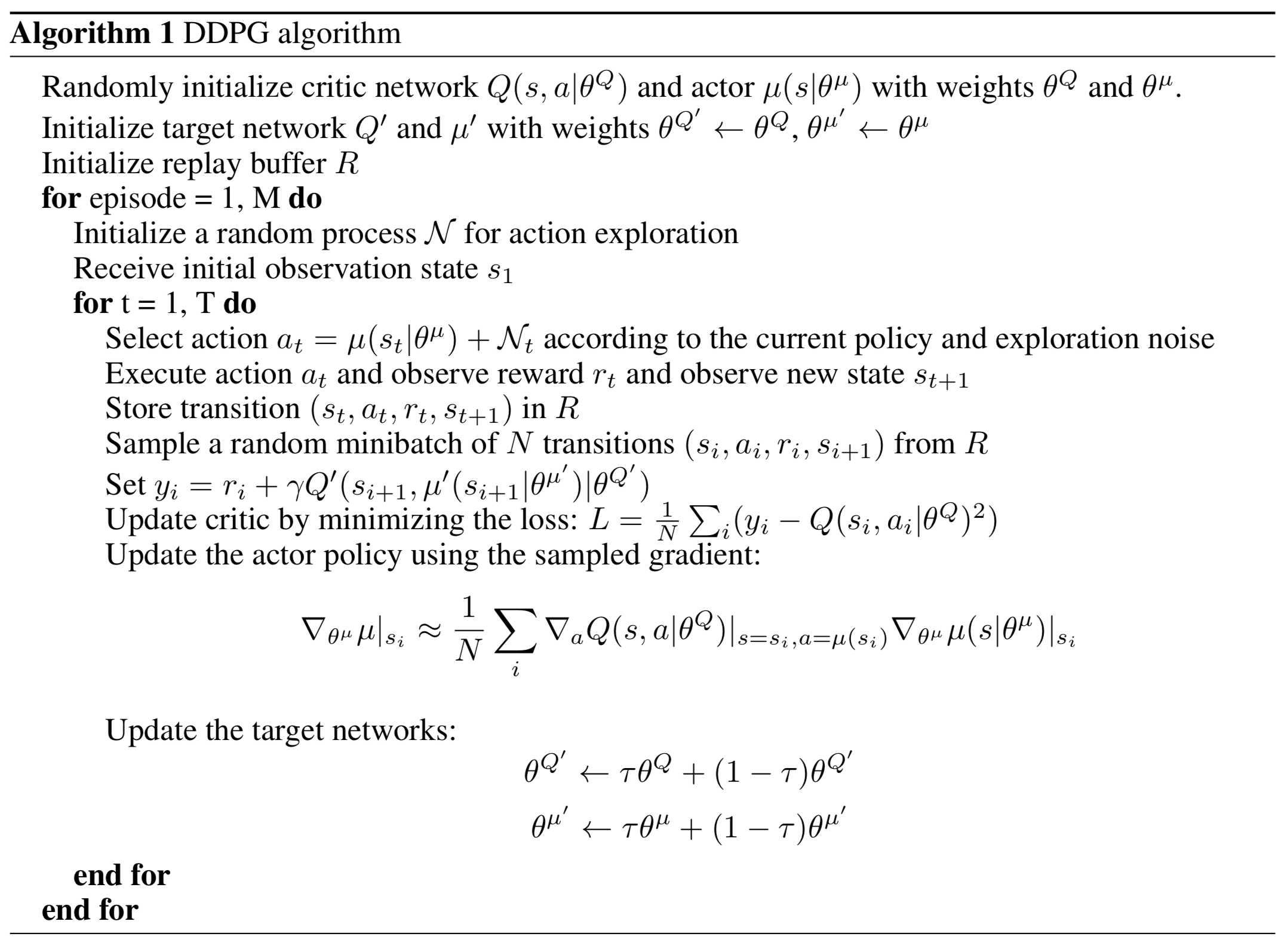
Typo: The loss for critic is
\[\begin{align} L={1\over N}\sum_i\left(y_i-Q\left(s_i, a_i|\theta^Q\right)\right)^2 \end{align}\]Heads up, the action taken by \( Q’ \) is different from that taken by \( Q \), the former is the action selected by the target actor, the latter is the action sampled along with the state \( s \).
Major Contribution
DDPG incorporates DQN into DPG so that the actor and critic can be represented by neural networks
Auxiliary Techniques
Batch Normalization
Different environments have different observations, which may vary dramatically. This makes it difficult for the network to learn effectively and to find hyper-parameters which generalize across environments with different scales of state values. Batch normalization helps to alleviate this problem by normalizing the input data
Gradually Update The Target Network
Instead of updating the target network every \( C \) steps, Here DDPG updates the target network slowly at every step
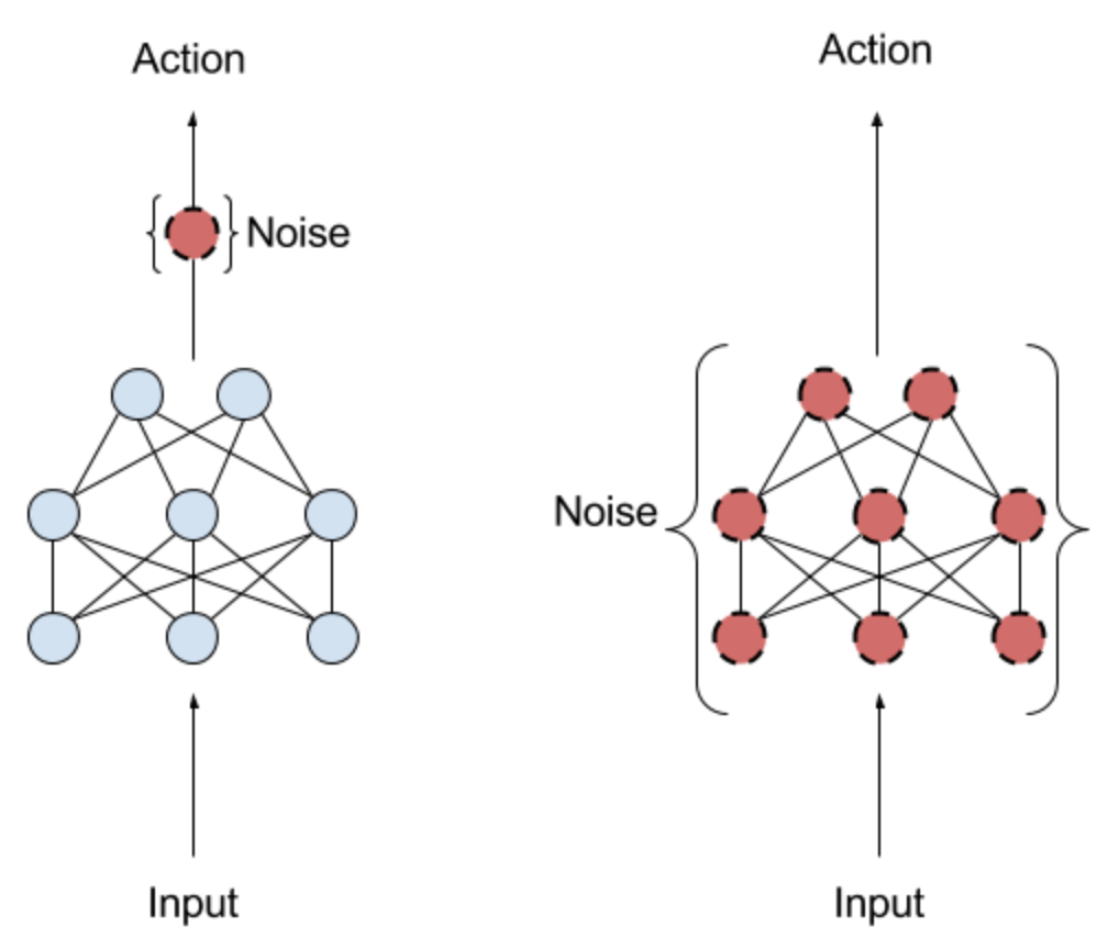
Noise
The above algorithm description adds exploration noise directly to action space. According to the research from openAI, however, adding adaptive noise to the parameters of the neural network rather than to action space helps boost performance
Hindsight Experience Reward
Algorithm
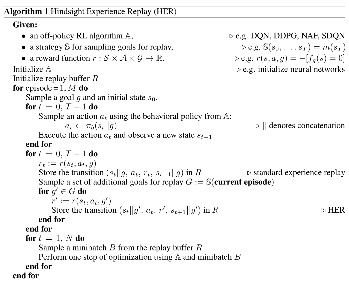
Major Contribution
HER introduces additional goals (as specified in the above algorithm) to improve the sample efficiency, and more importantly, thereby makes learning possible even if the reward signal is sparse and binary.
Additional goals are uniformly sampled from future states along the actual trajectory.
Sampling with HER Replacement
In the implementation provided by OpenAI, it stores in the replay buffer only the original transitions but not the transitions introduced by HER. After sampling a batch of transitions from the replay buffer, it then substitutes some of the samples with HER replacement. In this way, it avoids the replay filled with hindsight transitions at the price of more running time.
Main References
-
Human-level control through deep reinforcement learning
-
Deterministic policy gradient algorithms
-
Continuous control with deep reinforce learning
-
Hindsight experience replay