
Introduction
In the vanilla deep Q network, we store transitions in a replay buffer and then randomly sample from the buffer to improve our network. This strategy improves the data efficiency and stabilizes the learning process by breaking the temporal correlations between consecutive transitions (see my previous post for details). However, such a uniformly sampling process treats all transitions equally, ignoring the difference in their contributions to the learning process. Tom Schaul et al. in 2016 proposed prioritized replay, which prioritizes transition so as to sample more those transitions contributing more to the learning process.
There are two prioritized-replay strategies:
- Greedy prioritization: in which we sample transitions greedily with their priority (e.g., the largest absolute TD-error).
- Stochastic prioritization: in which we sample transitions with probability proportional to their priority
Greedy Prioritization
The advantage of the greedy prioritization is obvious:
- It’s easily implemented — a simple priority queue could do the job
- It frequently utilizes the transitions with a large TD error (since a TD error indicates how unexpected the corresponding transition is, and thereby provides a way to scale the potential improvement. This could be a poor estimate in some circumstances as well, e.g., when rewards are noisy. For now, we just make do with it.)
There are some issues with the greedy prioritization:
- It’s sensitive to noise spikes (e.g., when rewards are stochastic), which can be exacerbated by bootstrapping, where approximation errors appear as another source of noises.
- It focuses on a small subset of the transition: transitions with an initially high TD error get replayed frequently, whereas transitions with a low TD error on the first visit may not be replayed for a long time, which happens more frequently when errors shrink slowly (e.g., when using function approximation). This lack of diversity that makes the system prone to overfitting.
Stochastic Prioritization
A stochastic prioritized sampling method ensures the probability of being sampled is monotonic in a transition’s priority, while guaranteeing a non-zero probability even for the lowest-priority transition. The probability of sampling transition \( i \) is defined as
\[\begin{align} P(i)={p_i^\alpha\over\sum_kp_k^\alpha} \tag {1} \end{align}\]where \( p_i>0 \) is the priority of transition \( i \). The exponent \( \alpha \) determines how much prioritization is used, with \( \alpha=0 \) corresponding to the uniform case.
There are two variants of \( p_i \):
- \( p_i=\vert \delta_i\vert +\epsilon \), where \( \delta_i \) is the TD error of transition \( i \) and \( \epsilon \) is a small positive constant that prevents the edge-case of transitions not being visited once their error is zero
- \( p_i={1\over \mathrm{rank}(i)} \), where \( \mathrm{rank}(i) \) is the rank of transition \( i \) when the replay memory is sorted according to \( \vert \delta_i\vert \)
In practice, both distributions are monotonic in \( \vert \delta\vert \) and perform similarly. There are some theoretically arguments over these two variants: The latter is likely to be more robust, as it is insensitive to outliners and error magnitude. However, the ranks make the algorithm blind to the relative error scales, which could incur a performance drop when there is structure in the distribution of errors to be exploited, such as in sparse reward scenarios.
Implementation of Proportional Prioritization
The proportional prioritization is built on the sum-tree data structure, where every leaf node stores the priority for each individual transition, and the internal nodes sum up the priorities of their own children. At the update stage, we update the corresponding leaf node and propagate its priority to its parents. At the sampling stage, we divide the total priorities into \( k \) ranges(assuming we want to sample \( k \) transitions), randomly sampling a number at each range, walking down the sum-tree to locate the leaf node.
As an example of proportional sampling, assume we have a sum-tree as below:
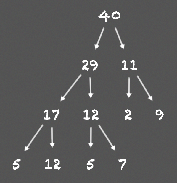
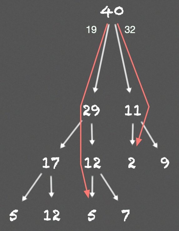
where numbers in the tree indicate the priorities of nodes. To randomly sample \( 2 \) leaf nodes, we first compute \( 2 \) ranges: \( [0, 20] \), \( [20, 40] \), then we randomly sample two values, one from each range. Let’s say we get \( 19 \), \( 32 \). The following image shows the route and the leaf nodes these two values end up
Implementation of Rank-Based Prioritization
In the implementation of the rank-based prioritization, we store transitions in a priority queue implemented with an array-based binary heap using indexes as priorities. This array-based heap is used as an approximation of a sorted array, which is infrequently sorted once every heap size(e.g., \( 10^6 \)) steps to prevent the heap becoming too unbalanced. Then we compute the probability as \( (1) \) suggests. At last, we divide the heap into \( k \) segments of equal probability. This process achieves three potential properties:
- The segment boundaries is precomputed, they change only when \( N \) or \( \alpha \) change
- The number of transitions in each segment is in inverse proportion to the priorities of the transitions in it.
- It works particularly well when \( k \) is the mini-batch size, in which we randomly sample one transition from each segment.
Annealing The Bias
The introduction of prioritized replay produces a bias towards transitions of high priority, which may lead to overfitting in a similar sense as the greedy prioritization (i.e. the model may overfit data with large priorities). We can correct this bias by using importance sampling weights
\[\begin{align} w_i=\left(p_{uniform}(i)\over p_{prioritized}(i)\right)^\beta=\left({1\over N}\cdot{1\over P(i)}\right)^\beta \end{align}\]This fully compensates for the non-uniform probability \( P(i) \) if \( \beta = 1 \). These weights can be folded into the Q-learning update by using \( w_i\delta_i ^2\) instead of \( \delta_i^2 \), where \( \delta_i \) is the TD error (it is thus weighted importance sampling. On the contrary, ordinary importance sampling only apply weight to the target, not the TD error. Mahmood et al. [2]). For stability reason, we always normalize weights by \( 1/\max_iw_i \) so as to avoid potentially increasing step size by \(w_i\). Furthermore, as \( \beta \) approaches \( 1 \), the normalization term grows, which helps to reduce step size in a similar way to exponential decay.
In typical reinforcement learning scenarios, the unbiased nature of the updates is most important near convergence at the end of training, but not in the process, since the process is highly non-stationary anyway, due to changing policies, state distributions, and bootstrap targets. Therefore, in practice, we linearly anneal \( \beta \) from its initial value to \( 1 \) at the end of learning.
Prioritization makes sure high-error transitions are seen many times. Importance sampling weights these transitions less, thereby helping reduce the gradient magnitude, allowing the algorithm to follow the curvature of highly non-linear optimization landscapes because the Taylor expansion is constantly re-approximated.
Discussion
PER does not help much for simple consistent environments(sometimes it may even impair the performance because of the bias introduced), but it indeed pays off for challenging tasks, such BipedalWalkerHardcore-v2, where some transitions provide more valuable information than others.
References
[1] Tom Schaul et al. Prioritized Experience Replay
[2] A. Rupam Mahmood et al. Weighted importance sampling for off-policy learning with linear function approximation