
Introduction
Reinforcement learning algorithms are sensitive to the choice of hyperparameters and typically require significant effort to identify hyperparameters that perform well on a new domain. much work has been done to ease hyperparameter tuning. For example, IMPALA, FTW, and AlphaStar resort to population-based training(PBT) to evolve hyperparameters from a group of agents training in parallel, showing great success in evolving hyperparameters during training. However, PBT usually requires a significantly large amount of computational resources to train a family of agents. In this post, we discuss a meta-gradient algorithm, called Self-Tuning Actor-Critic(STAC) introduced by Zahavy et al. 2020, that self-tunes all the differentiable hyperparameters of an actor-critic loss function.
Preliminaries
As Self-Tuning Actor-Critic(STAC) builds upon IMPALA, we briefly cover the loss functions used in IMPALA first
\[\begin{align} \mathcal L(\theta)=&g_V\mathcal L_V(\theta)+g_p\mathcal L_\pi(\theta)+g_e\mathcal L_{\mathcal H}(\theta)\\\ \mathcal L_V(\theta)=&\mathbb E_\mu[(v(x_t)-V_\theta(x_t))^2]\\\ \mathcal L_\pi(\theta)=&-\mathbb E_{(x_t,a_t,x_{t+1})\sim\mu}[\rho_t(r_t+\gamma v(x_{t+1})-V(x_t))\log\pi_\theta(a_t|x_t)]\\\ \mathcal L_{\mathcal H}(\theta)=&-\mathcal H(\pi_\theta) \end{align}\tag 1\]where the target value \(v(x_t)\) is defined by the V-trace.
\[\begin{align} v(x_t) :=& V(x_t)+\sum_{k=t}^{t+n-1}\gamma^{k-t}\left(\prod_{i=t}^{k-1}c_i\right)\delta_kV\\\ \delta_kV:=&\rho_k(r_k+\gamma V(x_{k+1})-V(x_k))\\\ c_{i}:=&\lambda \min\left(\bar c, {\pi(a_i|x_i)\over \mu(a_i|x_i)}\right)\\\ \rho_k:=&\min\left(\bar\rho, {\pi(a_k|x_k)\over \mu(a_k|x_k)}\right) \end{align}\]In STAC, we divide the hyperparameters into two groups: tunable hyperparameters and untunable hyperparameters. The tunable hyperparameters (aka meta-parameters) are a subset of differentiable hyperparameters—in the case of STAC, they’re \(\eta={\gamma,\lambda,g_V,g_p,g_e}\). As we’ll see in the next section, these meta-parameters are differentiable from an outer meta-objective through inner gradients.
Self-Tuning Actor-Critic
STAC self-tunes all the meta-parameters following the meta-gradient framework, which involves an inner loop and an outer loop. In the inner loop, STAC optimizes Equation \((1)\) by taking one step gradient descent w.r.t. \(\mathcal L\) parameterized by the meta-parameter \(\eta\) as in IMPALA: \(\tilde\theta(\eta)=\theta-\alpha\nabla_\theta\mathcal L(\theta,\eta)\). In the outer loop, we cross-validate the new parameters on a subsequent, independent sample—though, in practice, we use the same sample in both loops for efficient learning—utilizing a differentiable meta-objective \(\mathcal L_{outer}(\tilde\theta(\eta))\). Specifically, the meta-objective adopted by STAC is
\[\begin{align} \mathcal L_{outer}(\tilde\theta(\eta))=g_V^{outer}\mathcal L_V(\theta)+g_p^{outer}\mathcal L_\pi(\theta)+g_e^{outer}\mathcal L_{\mathcal H}(\theta)+g_{kl}^{outer}D_{KL}(\pi_{\tilde\theta(\eta)},\pi_\theta)\tag 2 \end{align}\]where \((\gamma^{outer},\lambda^{outer},g_V^{outer}, g_p^{outer},g_e^{outer}, g_{kl}^{outer})\) are hyperparameters. For Atari games, they are \((0.995, 1, 0.25, 1, 0.01, 1)\). Zahavy et al. 2020 does not explain the motivation of the KL loss, but they do find that \(g_{kl}^{outer}=1\) improves the performance. As it regularizes the updated policy against its previous version, one can regard it as a regularization technique imposed by meta-gradient. That is, we want to learn meta-gradient such that the inner gradient step does not make a big change to our policy.
The gradients of \(\eta\) are computed by differentiating \(\mathcal L_{outer}(\tilde\theta(\eta))\) through \(\nabla_\theta\mathcal L(\theta,\eta)\). That is,
\[\begin{align} \nabla_{\eta}\mathcal L_{outer}(\tilde\theta(\eta))=&\nabla_\eta{\tilde\theta(\eta)}\nabla_{\tilde\theta(\eta)}\mathcal L_{outer}({\tilde\theta(\eta)})\\\ =&-\alpha\nabla_\eta\nabla_\theta\mathcal L(\theta,\eta)\nabla_{\tilde\theta(\eta)}\mathcal L_{outer}({\tilde\theta(\eta)})\tag 3 \end{align}\]To ensure that all the meta-parameters are bounded, we apply sigmoid on all of them. We also multiply the loss coefficient \((g_V,g_p,g_e)\) by the respective coefficient in the outer loss to guarantee that they are initialized from the same values. For example \(\gamma=\sigma(\gamma)\), \(g_V=g_V^{outer}\sigma(g_V)\). We initialize all the meta-parameters to \(\eta^{init}=4.6\) such that \(\sigma(\eta^{eta})=0.99\). This guarantees that the inner loss is initialized to be (almost) the same as the outer loss.
Leaky V-trace
As we’ve discussed in the previous posts([1], [2]), the fixed policy of the V-trace operator is controlled by the hyperparameter \(\bar\rho\)
\[\begin{align} \pi_{\bar\rho}(a|x)={\min(\bar\rho\mu(a|x),\pi(a|x))\over{\sum_{b\in A}\min(\bar\rho\mu(b|x),\pi(b|x))}} \end{align}\]The truncation level \(\bar c\) controls the speed of convergence by trading off variance reduction for convergence rate. Though importance weight clipping effectively reduces the variance, it weakens the effect of later TD errors and worsens the contraction rate. Noticing that, Zahavy et al. 2020 propose leaky V-trace that interpolates between the truncated importance sampling and canonical importance sampling. Leaky V-trace uses the same target value as V-trace except that
\[\begin{align} c_{i}:=&\lambda \big(\alpha_c\min(\bar c, \text{IS}_t)+(1-\alpha_c)\text{IS}_t\big)\\\ \rho_k:=&\alpha_\rho\min(\bar\rho, \text{IS}_t)+(1-\alpha_\rho)\text{IS}_t\\\ where\quad \text{IS}_t=&{\pi(a_i|x_i)\over \mu(a_i|x_i)} \end{align}\]Where \(\alpha_c\) and \(\alpha_\rho\) are introduced to allow the importance weights to “leak back” creating the opposite effect to clipping
Theorem 1 below shows that Leaky V-trace converges to \(V^{\pi_{\bar\rho},\alpha_\rho}\)
Theorem 1. Assume that there exists \(\beta\in(0,1]\) such that \(\mathbb E_\mu\min(\bar\rho, IS_t) \ge\beta\). Then the operator \(\mathcal R\) has a unique fixed point \(V^{\pi_{\bar\rho,\alpha_\rho}}\), which is the value function of the policy \(\pi_{\bar\rho,\alpha_\rho}\) defined by
\[\begin{align} \pi_{\bar\rho,\alpha_\rho}={\alpha_\rho\min(\bar\rho\mu(a|x),\pi(a|x))+(1-\alpha_\rho)\pi(a|x)\over \alpha_\rho\sum_b\min(\bar\rho\mu(b|x),\pi(b|x))+(1-\alpha_\rho)}\tag 4 \end{align}\]Furthermore, \(\mathcal R\) is an \(\eta\)-contraction mapping in sup-norm with
\[\begin{align} \eta:=\gamma^{-1}-(\gamma^{-1}-1)\mathbb E_\mu\left[\sum_{k\ge t}\gamma^{k-t}\left(\prod_{i=t}^{k-2}c_i\right)\rho_{k-1}\right]\le 1-(1-\gamma)(\alpha_\rho\beta+1-\alpha_\rho)< 1\tag 5 \end{align}\]The proof follows the proof of V-trace with small adaptations for the leaky V-trace coefficient. We leave it to the Supplementary Materials
Theorem 1 requires \(\alpha_\rho\ge \alpha_c\), and STAC parameterizes them with a single parameter \(\alpha=\alpha_\rho=\alpha_c\) and includes it in meta-parameters—\(\alpha\) is initialized to \(1\) and the outer loss is fixed to be V-trace, i.e. \(\alpha^{outer}=1\).
STAC with Auxiliary Tasks
Zahavy et al. 2020 further introduce an agent that extends STAC with auxiliary policy and value heads. The motivation is to utilize meta-gradient to learn different hyperparameters for different policy value heads. For example, auxiliary objectives with different discount factors allow STACX to reason about multiple horizons. In practice, however, these heads serve more like auxiliary tasks as none of them are actually used to sample trajectories; sampling trajectories using auxiliary policies—even with some ensemble techniques—compromises the learning of the main policy. This is most likely caused by the choice of the V-trace loss as way off-policy data causes the V-trace operator to converge to value function of policy different from the optimal one.
On account of the introduction of policy and value heads, the meta-parameters for STACX now becomes \(\eta={\gamma^i,\lambda^i,g_V^i,g_p^i,g_e^i,\alpha^i}_{i=1}^3\). On the other hand, the outer loss does not change; it is still defined only w.r.t. the main heads.
Universal Value Function Approximation for Meta-Parameters
Xu et al. 2018 in Section 1.4 point out that the target function \(v(x_t)\) is non-stationary, adapting along with the meta-parameters throughout the training process. As a result, there is a danger that the value function \(v_\theta\) becomes inaccurate, since it may be approximating old returns. For example, when \(\gamma\) changes from \(0\) to \(1\), the value function learned for \(\gamma=0\) does no longer provide a valid approximation.
To deal with non-stationarity in the value function and policy, we turn to universal value function approximation, where we provide the meta-parameter \(\eta\) as an additional input the condition the value function and policy, as follows:
\[\begin{align} V_\theta^\eta(s)=&V_\theta([s;e_\eta])\\\ \pi_\theta^\eta(s)=&\pi_\theta([s;e_\eta])\\\ e_\eta=&W_\eta\eta \end{align}\]where \(e_\eta\) is the embedding of \(\eta\), \([s;e_\eta]\) denotes the concatenation of vectors \(s\) and \(e_\eta\). \(W_\eta\) is the learnable embedding matrix.
Experimental Results
Effect of self-tuning and auxiliary tasks
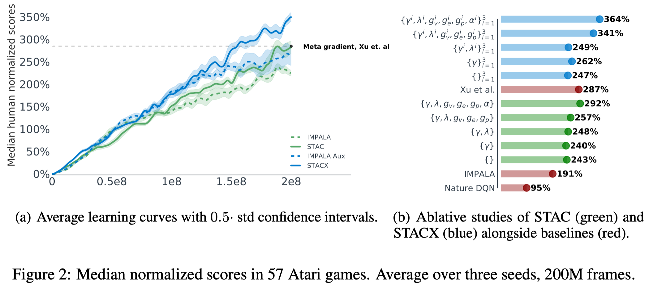
Figure 2 shows that both self-tuning and auxiliary tasks improve the performance. Furthermore, Figure. 2(b) shows that leaky V-trace performs better than V-trace. Noticeably, auxiliary tasks do not bring much performance gain when self-tuning is completely off.
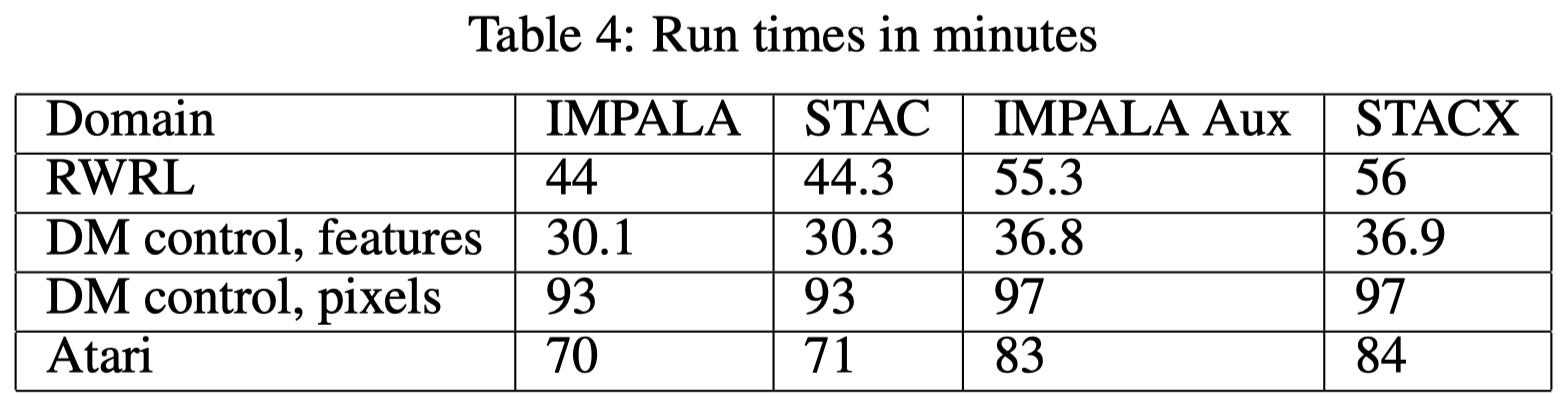
Table 4 shows that self-tuning does not incur many overheads while auxiliary tasks increase the run time by a noticeable margin. Another experiment with multiple CPU workers and a single GPU learner tells a different story. In that case, STAC requires about \(25\%\) more time, while the extra run time from the auxiliary tasks is negligible.
Adaptivity of meta-parameters
Zahavy et al. further monitor the evolution of meta-parameters during training. We summarize several interesting observations below
- The meta-parameters of the auxiliary heads are self-tuned to have relatively similar values but different than those of the main head. For example, the main head discount factor converges to \(0.995\). In contrast, the auxiliary heads’ discount factors often change during training and get to lower values.
- The leaky V-trace parameter \(\alpha\) is close to \(1\) at the beginning but may self-tune near the end of the training depending on the task.
- When we let \(\alpha_\rho\) and \(\alpha_c\) tune separately, STACX self-tunes \(\alpha_\rho\ge\alpha_c\) most of the time.
References
Zahavy, Tom, Zhongwen Xu, Vivek Veeriah, Matteo Hessel, and Junhyuk Oh. 2020. “A Self-Tuning Actor-Critic Algorithm,” no. 1: 1–34.
Xu, Zhongwen, Hado Van Hasselt, and David Silver. 2018. “Meta-Gradient Reinforcement Learning.” Advances in Neural Information Processing Systems 2018-December: 2396–2407.
Supplementary Materials
Analysis of Leaky V-trace
Theorem 1. Assume that there exists \(\beta\in(0,1]\) such that \(\mathbb E_\mu\min(\bar\rho, IS_t) \ge\beta\). Then the operator \(\mathcal R\) has a unique fixed point \(V^{\pi_{\bar\rho,\alpha_\rho}}\), which is the value function of the policy \(\pi_{\bar\rho,\alpha_\rho}\) defined by
\[\begin{align} \pi_{\bar\rho,\alpha_\rho}={\alpha_\rho\min(\bar\rho\mu(a|x),\pi(a|x))+(1-\alpha_\rho)\pi(a|x)\over \alpha_\rho\sum_b\min(\bar\rho\mu(b|x),\pi(b|x))+(1-\alpha_\rho)}\tag 4 \end{align}\]Furthermore, \(\mathcal R\) is an \(\eta\)-contraction mapping in sup-norm with
\[\begin{align} \eta:=\gamma^{-1}-(\gamma^{-1}-1)\mathbb E_\mu\left[\sum_{k\ge t}\gamma^{k-t}\left(\prod_{i=t}^{k-2}c_i\right)\rho_{k-1}\right]\le 1-(1-\gamma)(\alpha_\rho\beta+1-\alpha_\rho)< 1\tag 5 \end{align}\]Proof. As in the analysis of V-trace, we can write the Leaky V-trace operator as
\[\begin{align} \mathcal R V(x_t)=(1-\mathbb E_\mu\rho_t)V(x_t)+\mathbb E_\mu\left[\sum_{k\ge t}\gamma^{k-t}\left(\prod_{i=t}^{k-1}c_i\right)\big(\rho_kr_k+\gamma(\rho_k-c_k\rho_{k+1})V(x_{k+1})\big)\right] \end{align}\]where we move \(-\rho_{k+1}V(x_{k+1})\) in \(\delta_{k+1}V\) into \(\delta_{k}V\). Therefore, we have
\[\begin{align} \mathcal RV_1(x_{t})-\mathcal RV_2(x_t)&=(1-\mathbb E_\mu\rho_t)(V_1(x_t)-V_2(x_t))+\mathbb E_\mu\left[\sum_{k\ge t}\gamma^{k-t+1}\left(\prod_{i=t}^{k-1}c_i\right)\big((\rho_k-c_k\rho_{k+1})(V_1(x_{k+1})-V_2(x_{k+1})\big)\right]\\\ &=\mathbb E_\mu\left[\sum_{k\ge t}\gamma^{k-t}\left(\prod_{i=t}^{k-2}c_i\right)\big(\underbrace{(\rho_{k-1}-c_{k-1}\rho_{k})}_{a_k}(V_1(x_{k})-V_2(x_{k})\big)\right] \end{align}\]with the notation that \(c_{t-1}=\rho_{t-1}=1\) and \(\prod_{i=t}^{k-2}c_i=1\) for \(k=t\) and \(t+1\).
We shall see that \(a_k\ge0\) in expectation as \(\bar\rho\ge\bar c\) and \(\alpha_\rho\ge \alpha_c\) and we have
\[\begin{align} \mathbb E_\mu a_k\ge\mathbb E_\mu[\rho_{k-1}(1-\rho_k)]\ge 0 \end{align}\]since \(\mathbb E_\mu\rho_k=\alpha_\rho\mathbb E_\mu[\min(\bar\rho, \text{IS}t)+(1-\alpha\rho)\text{IS}t]\le \alpha\rho+(1-\alpha_\rho)=1\). Thus \(V_1(x_{t})-V_2(x_t)\) is a linear combination of the values \(V_1-V_2\) at other states, weighted by non-negative coefficients whose sum is
\[\begin{align} &\sum_{k\ge t}\gamma^{k-t}\mathbb E_\mu\left[\left(\prod_{i=t}^{k-2}c_i\right)(\rho_{k-1}-c_{k-1}\rho_{k})\right]\\\ =&\sum_{k\ge t}\gamma^{k-t}\mathbb E_\mu\left[\left(\prod_{i=t}^{k-2}c_i\right)\rho_{k-1}\right]-\sum_{k\ge t}\gamma^{k-t}\mathbb E_\mu\left[\left(\prod_{i=t}^{k-1}c_i\right)\rho_{k}\right]\\\ &\qquad\color{red}{\text{add }\gamma^{-1}(\mathbb E_{\mu}\rho_{t-1}-1)\text{ to the second term and rearange}}\\\ =&\sum_{k\ge t}\gamma^{k-t}\mathbb E_\mu\left[\left(\prod_{i=t}^{k-2}c_i\right)\rho_{k-1}\right]-\gamma^{-1}\left(\sum_{k\ge t}\gamma^{k-t}\mathbb E_\mu\left[\left(\prod_{i=t}^{k-2}c_i\right)\rho_{k-1}\right]-1\right)\\\ =&\gamma^{-1}-(\gamma^{-1}-1)\sum_{k\ge t}{\gamma^{k-t}\mathbb E_\mu\left[\left(\prod_{i=t}^{k-2}c_i\right)\rho_{k-1}\right]}=\eta\\\ &\qquad\color{red}{\sum_{k\ge t}{\gamma^{k-t}\mathbb E_\mu\left[\left(\prod_{i=t}^{k-2}c_i\right)\rho_{k-1}\right]}\ge\sum_{k=t}^{t+1}{\gamma^{k-t}\mathbb E_\mu\left[\left(\prod_{i=t}^{k-2}c_i\right)\rho_{k-1}\right]}=1+\gamma\mathbb E_\mu\rho_t}\\\ &\qquad\color{red}{\gamma<1\text{ and }(\gamma^{-1}-1)>0}\\\ \le&\gamma^{-1}-(\gamma^{-1}-1)(1+\gamma\mathbb E_\mu\rho_t)\\\ =& 1-(1-\gamma)\mathbb E_\mu\rho_t\\\ &\qquad\color{red}{\mathbb E_\mu\rho_t\ge\beta}\\\ \le& 1-(1-\gamma)(\alpha_\rho\beta+1-\alpha_\rho)\\\ &\qquad\color{red}{\beta\in(0, 1]}\\\ \le&\gamma<1 \end{align}\]We deduce that \(\Vert\mathcal RV_1(x_t)-\mathcal RV_1(x_t)\Vert\le \eta\Vert V_1-V_2\Vert_\infty\), with \(\eta\) defined in Equation \((4)\), so \(\mathcal R\) is a contraction mapping. Thus \(\mathcal R\) possesses a unique fixed point. Let us now prove that this fixed point is \(V^{\pi_\bar\rho,\alpha_\rho}\). We have
\[\begin{align} &\mathbb E_\mu[\rho_t(r_t+\gamma V^{\pi_\bar\rho,\alpha_\rho}(x_{t+1})-V^{\pi_\bar\rho,\alpha_\rho}(x_t))|x_t]\\\ =&\sum_a\mu(a|x_t)\left(\alpha_\rho\min\left(\bar\rho, {\pi(a|x_t)\over \mu(a|x_t)}\right)+(1-\alpha_\rho){\pi(a|x_t)\over \mu(a|x_t)}\right)\left(r_t+\gamma\sum_{x_{t+1}} p(x_{t+1}|x_t,a)V^{\pi_\bar\rho,\alpha_\rho}(x_{t+1})-V^{\pi_\bar\rho,\alpha_\rho}(x_t)\right)\\\ =&\sum_a\left(r_t+\gamma\sum_{x_{t+1}} p(x_{t+1}|x_t,a)V^{\pi_\bar\rho}(x_{t+1})-V^{\pi_\bar\rho}(x_t)\right)\Big(\alpha_\rho\min(\bar\rho\mu(a|x_t), {\pi(a|x_t)})+(1-\alpha_\rho)\pi(a|x_t\big)\Big)\\\ =&\underbrace{\sum_a\pi_{\bar\rho,\alpha_\rho}(a|x_t)\left(r_t+\gamma\sum_{x_{t+1}} p(x_{t+1}|x_t,a)V^{\pi_\bar\rho}(x_{t+1})-V^{\pi_\bar\rho}(x_t)\right)}_{=0,\text{ since }V^{\pi_\bar\rho,\alpha_\rho}\text{ is the value function of }{\pi_{\bar\rho,\alpha_\rho}}}\sum_{b\in A}\Big(\alpha_\rho\min(\bar\rho\mu(b|x_t), {\pi(b|x_t)})+(1-\alpha_\rho)\pi(b|x_t\big)\Big)\\\ =&0 \end{align}\]Therefore \(\delta_kV^{\pi_\bar\rho,\alpha_\rho}=0\) and \(\mathcal RV^{\pi_\bar\rho,\alpha_\rho}=V^{\pi_\bar\rho,\alpha_\rho}\), i.e, \(V^{\pi_\bar\rho,\alpha_\rho}\) is the unique fixed point of \(\mathcal R\).