
Introduction
Model-free reinforcement learning has achieved super-human performance in many areas. However, the impractically large sample requirement makes it unsuitable for solving challenging real-world problems. Worse still, classic model-free RL can be extremely sample inefficient in tasks with sparse rewards, such as goal-directed tasks. Model-based RL improves sample efficiency by utilizing the rich information contained in state transition tuples to train a predictive model, but often does not achieve the same asymptotic performance as model-free RL due to model bias. In this post, we discuss temporal difference models (TDMs), a family of goal-conditioned value functions that can be trained with model-free learning and used for model-based control.
Cautions
Before we dive into the algorithm, one thing may be worth keeping in mind: TDMs are designed specifically for goal-directed tasks where the agent tries to reach some goal(or terminal) states. Once it achieves these states, it gets rewarded and the episode terminates. Later, we will see why this is the case.
Temporal Difference Model Learning
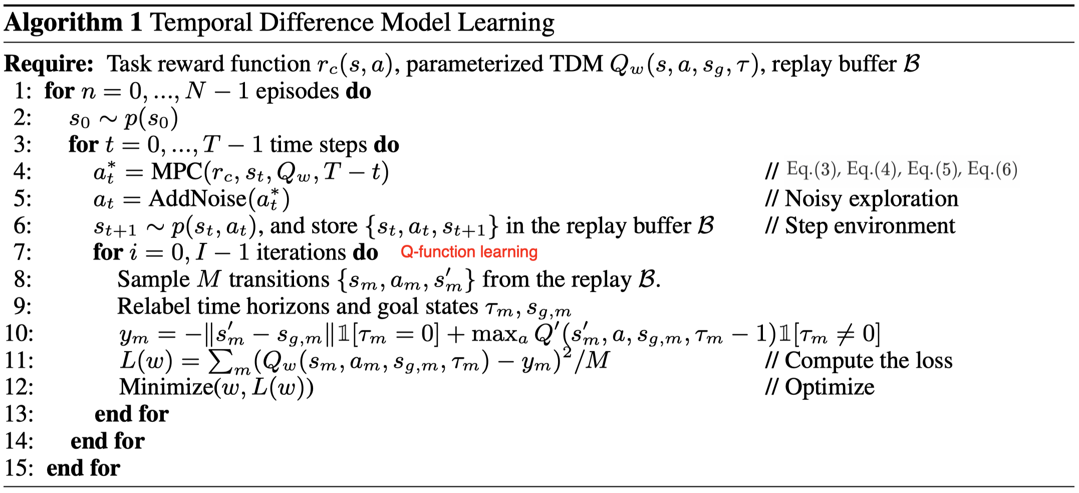
TDMs can be broken down into two parts: 1. Making decisions based on model-predictive control. 2. Learning \(Q\)-function. In this section, we will first define \(Q\)-function used in TDMs, then we discuss how TDMs make decisions using this \(Q\)-function. Next, we will come back to this \(Q\)-function, seeing how it is trained. This section ends with the complete algorithm summary.
TDM definition
The \(Q\)-function (a.k.a., TDM) is defined as,
\[\begin{align} Q(s_t,a_t,s_g,\tau)=\mathbb E_{p(s_{t+1}|s_t,a_t)}\big[-D(s_{t+1},s_g)\mathbf 1[\tau=0]+\max_aQ(s_{t+1},a,s_g,\tau-1)\mathbf1[\tau\ne0]\big]\tag {1} \end{align}\]which measures how close the agent, starting from state \(s_t\) with action \(a_t\), can get to \(s_g\) in \(\tau\) steps, if it acts optimally towards \(s_g\) according to the TDM. Note that this TDM differs from the classic \(Q\)-function in model-free RL in four aspects:
- It is a goal-conditioned value function augmented by the planning horizon \(\tau\). These extra parameters allow the method to relabel goals and horizons, whereby TMDs are able to learn from more training signals.
- It does not measure the expected future reward as usual, thus rewards from environment does not contribute to its learning. It, instead, adopts some distance metric as its reward function (i.e., \(r_d(s_t,a_t,s_{t+1},s_g)=-D(s_{t+1},s_g)\), where \(D(s_{t+1},s_g)\) is a distance function, such as L1 norm \(\Vert s_{t+1}-s_g\Vert\) employed by Pong et al. in their experiments, or the Euclidian distance).
- The maximal reward \(r_d(s_{t+\tau},a_{t+\tau},s_{t+\tau+1},s_g)\) back-propagates into \(Q(s_t,a_t,s_g,\tau)\) — There is no intermediate reward cumulative in this function, or we could take it as if all intermediate rewards are zero.
- The TDM could use vector-valued rewards since it is not used as a measure of policy performance. Specifically, we could have the reward of the same dimensionality as state and each dimension of the reward measures the difference in that dimension of the state. This provides more training signals from each training point, and is found substantially boost sample efficiency.
Decision Making
For now, we assume the TDM can be well trained and only concentrate on how the TDM can help to make decisions, which also reveals the specific design of the TDM.
The algorithm relies on model-predictive control(MPC) to make decisions. Traditional MPC can be formalized as the following optimization problem
\[\begin{align} a_t=&\underset{a_{t:t+T}}{\arg\max}\sum_{i=t}^{t+T} r_c(s_i,a_i)\\\ where\quad s_{i+1}=&f(s_i,a_i)\ \forall i \in\{t,\dots,t+T-1\} \end{align}\]where \(r_c\) denotes the reward function provided by the environment and \(f\) denotes the dynamics model. We can also rewrite the dynamics constraint in the above equation in terms of an implicit dynamics
\[\begin{align} a_t=&\underset{a_{t:t+T}}{\arg\max}\sum_{i=t}^{t+T} r_c(s_i,a_i)\tag {2}\\\ such\ that\ C(s_i,a_i,s_{i+1})=&0\ \forall i \in\{t,\dots,t+T-1\} \end{align}\]where \(C(s_i,a_i,s_{i+1})=0\) iff \(s_{i+1}=f(s_i,a_i)\). It is easy to see that \(Q(s_i,a_i,s_{i+1},0)\) is in fact a valid choice of \(C\).
Now assume we only care about the reward at every \(K\) step. In that case, Eq.\((2)\) equals to
\[\begin{align} a_t=&\underset{a_{t:K:t+T},s_{t+K:K:t+T}}{\arg\max}\sum_{i=t,t+K,\dots,t+T} r_c(s_i,a_i)\tag {3}\\\ such\ that\quad Q(s_i,a_i,s_{i+K},K-1)=&0\quad \forall i \in\{t,t+K,\dots,t+T-K\} \end{align}\]As the TDMs become effective for longer horizons, we can increase \(K\) until \(K=T\), and plan over only a single effective time step:
\[\begin{align} a_t=&\underset{a_t,s_{t+T},a_{t+T}}{\arg\max}r_c(s_{t+T},a_{t+T})\tag{4}\\\ such\ that\quad Q(s_t,a_t,s_{t+T},T-1)=&0 \end{align}\]Notice that we does not take into account the intermediate rewards at all in the above optimization problem, this explains why we said TMDs were designed for goal-directed tasks.
Although Eq.\((4)\), the optimal control formulation, drastically reduces the number of states and actions to be optimized for long-term planning, it requires solving a constrained optimization problem(one may solve it with recourse to Augmented Lagrangian Method), which is more computationally expensive than unconstrained problems. The authors propose a specific architectural decision in the design of the \(Q\)-function to remove the need for constrained optimization. Specifically, the \(Q\)-function is defined as \(Q(s,a,s_g,\tau)=-\vert f(s,a,s_g,\tau)-s_g\vert \), where \(f(s,a,s_g,\tau)\) is trained to explicitly predict the state that will be reached in \(\tau\) steps by a policy attempting to reach \(s_g\). This model can then be used to choose the action with fully explicit MPC as below
\[\begin{align} a_t=\underset{a_t,s_{t+T},a_{t+T}}{\arg\max} r_c(f(s_t,a_t,s_{t+T},T),a_{t+T})\tag {5} \end{align}\]It is important to notice that we do not use \(s_g\) in \(f\) above, since we do not know which goal state results in the best outcome. In the case where the task is to reach a single goal state \(s_g\) and there is no need to distinguish different reward signal, a simpler approach to extract a policy is to use the TDM directly:
\[\begin{align} a_t=\underset{a}{\arg\max}Q(s_t,a,s_g,T)\tag {6} \end{align}\]TDM Learning
The goal-conditioned nature of TDM makes it possible to relabel goals. One suggested strategy is to uniformly sample future states along the actual trajectory in the buffer (i.e., for \(s_t\), choose \(s_g=s_{t+k}\) for a random \(k>0\)). We also sample the horizon \(\tau\) uniformly at random between \(0\) and the maximum horizon \(\tau_\max\). Then, for each relabelled time horizon and goal state \(\tau_m\), \(s_{g,m}\), we compute the target as follows
\[\begin{align} y_m=-|s_{t+1}-s_{g,m}|\mathbf 1[\tau_m=0]-|f(s_{t+1},a^\*,s_{g,m},\tau_m-1)-s_{g,m}|\mathbf 1[\tau_m\ne 0]\\\ where\ a^\*=\underset{a}{\arg\max}Q(s_{t+1},a,s_{g,m},\tau_m-1) \end{align}\]where \(\vert \cdot\vert \) is the absolute difference in each dimension or L1 norm depending on whether the TDM is vector-valued or scalar.
Algorithm
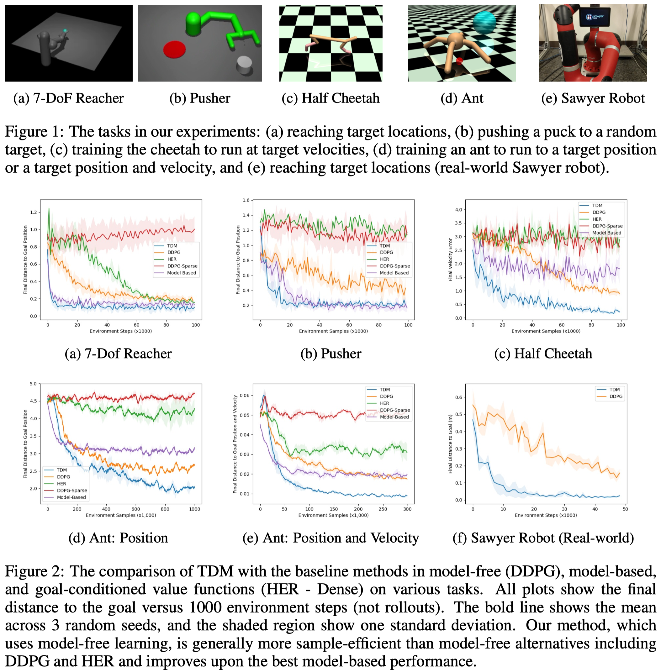
Experimental Results
Discussion
Why is TDMs able to achieve asymptotically better performance than traditional model-based RL?
Two possible reasons:
- Goal-conditioned vector-valued value functions provide more training signal to the model. As a result, the learned model is more robust than models learned by a traditional model-based algorithm.
- The number of states and actions involved in MPC is reduced. Therefore, there is less place on which the model bias can be imposed.
Why is \(Q\)-learning in TDMs more sample efficient than tranditional off-policy algorithms in sparse reward environments?
There are much more training signals in TDMs thanks to the definition of the \(Q\)-function:
- Rewards are defined as a distance function, not from the environment, so the reward signal could actually be pretty dense;
- Rewards and \(Q\)-function in TDMs are vector-valued;
- \(Q\)-function in TDMs is conditioned on the goal and horizon, and we constantly relabel time horizons and goal states during training.
Why can TDMs be trained with any off-policy Q-learning algorithm?
We can take the TDM as a \(Q\)-function learned in an environment where rewards are only given every \(\tau\) steps. In this way, we can see that the TDM is in fact a well-defined undiscounted \(Q\)-function.
References
Vitchyr Pong et al. Temporal Difference Models: Model-Free Deep RL for Model-Based Control
Code: https://github.com/vitchyr/rlkit