SAC-X — Scheduled Auxiliary Control

Introduction

We discuss Scheduled Auxiliary Control (SAC-X), a new learning paradigm in the context of Reinforcement Learning (RL). SAC-X enables learning of complex behaviors – from scratch – in the presence of multiple sparse reward signals. To this end, the agent is equipped with a set of general auxiliary tasks, that it attempts to learn simultaneously via off-policy RL. The key idea behind this method is that active (learned) scheduling and execution of auxiliary policies allows the agent to efﬁciently explore its environment – enabling it to excel at sparse reward RL. Experiments in several challenging robotic manipulation settings demonstrate the power of this approach. A video of the rich set of learned behaviors can be found at https://youtu.be/mPKyvocNe_M. (Abstraction from the original paper, since I figured it was extremely concise.)

Preliminaries

Consider a sparse reward problem as finding the optimal policy \(\pi^*\) in an MDP \(\mathcal M\) with a reward function characterized by an \(\epsilon\) region in state space. That is, we have

\[\begin{align} r_{\mathcal M}(s,a)= \begin{cases}\delta_{s_g}(s)&d(s,s_g)\le\epsilon\\\ 0&else \end{cases} \end{align}\]

where \(s_g\) denotes a goal state and \(d(s,s_g)\) denotes the distance between the goal state and state \(s\). In practice, we could have \(d(s,s_g)=\Vert s-s_g\Vert_2\), which defines a sphere space around \(s_g\).

In addition to the main MDP \(\mathcal M\), we further design a set of auxiliary MDPs \(\mathcal A={\mathcal A_1,\dots,\mathcal A_K}\) that share the state, observation and action space as well as the transition dynamics with \(\mathcal M\). Together, we have \(\mathfrak T=\mathcal A\cup{\mathcal M}\). We further assume full control over the auxiliary rewards; i.e., we assume knowledge of how to compute auxiliary rewards and assume we can evaluate them at any state action pair.

Scheduled Auxiliary Control

Overview

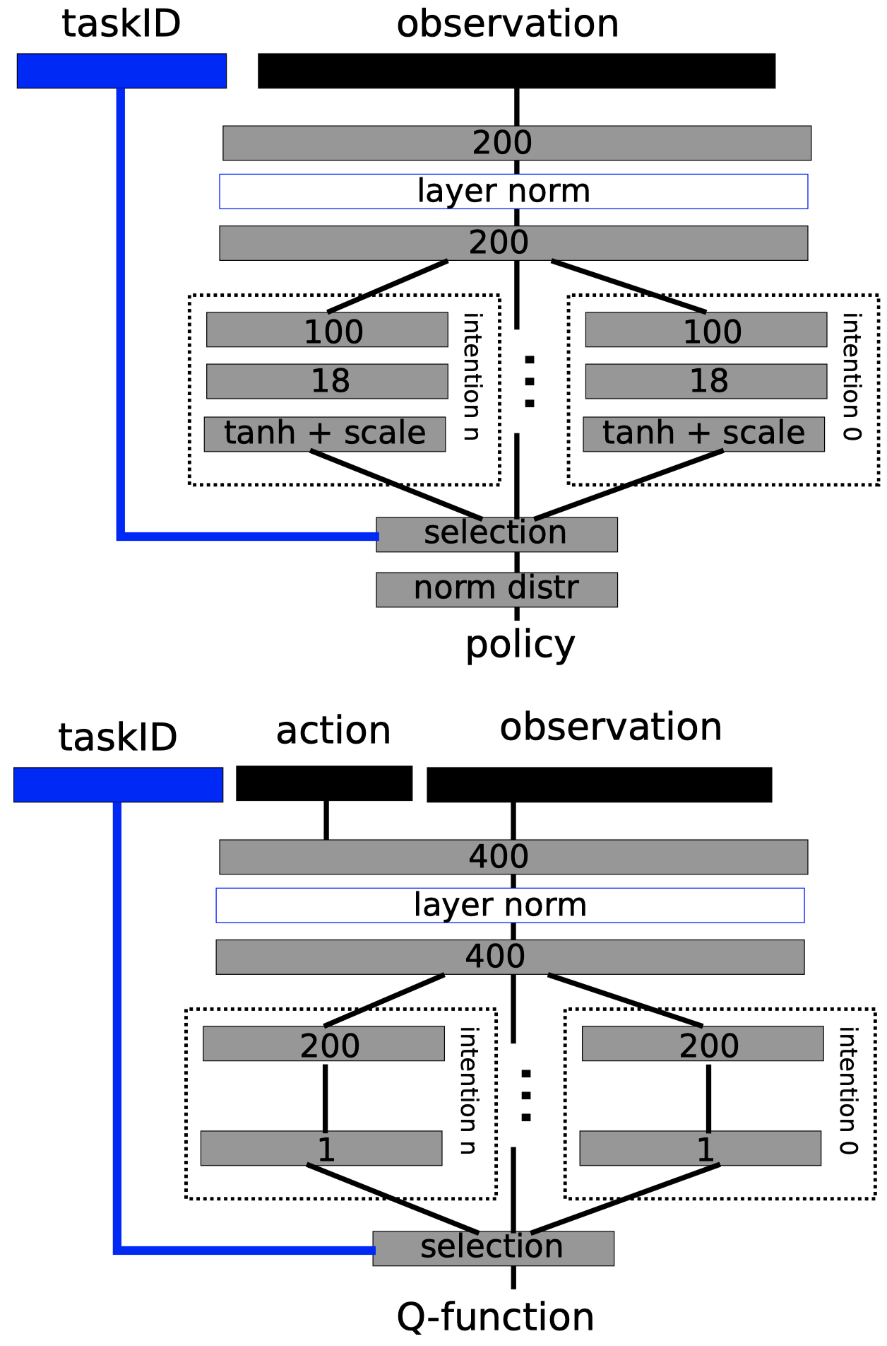
Scheduled Auxiliary Control(SAC-X) mainly consists of three components: a policy(a.k.a. intention) and a \(Q\)-function for each task, and a scheduler that sequences intention-policies. An example of the network architecture is given on the right.

Now we roughly describe the training workflow: Every \(\xi\) steps(\(\xi=150\) in their experiments) in an episode, the scheduler selects an MDP \(\mathcal T\in\mathfrak T\) and the agent takes the corresponding policy \(\pi_{\mathcal T}(a\vert s)\) afterward. Meanwhile, network updates are done simultaneously, in a background thread or by some parameter server as we will see later.

In the rest of this section, we will further elaborate each component but you may find something that is not consistent with those in the paper. Be cautious about the places followed by \(^*\). I boldly modify these details since I found those in the paper are somewhat confusing.

\(Q\)-function

Since no policy runs an entire episode, it is necessary to learn each intention \(\pi_{\mathcal T}(a\vert s)\) in an off-policy fashion so that policies can be applied to any state in the state space. As a result, \(Q\)-functions are required to predict future rewards under each intention. The authors employ Retrace for off-policy evaluation of all intentions. Concretely, we train \(Q\)-functions \(Q_{\mathcal T}(s,a;\phi)\) by minimizing the following loss:

\[\begin{align} \min_\phi\mathcal L(\phi)&=\mathbb E_{(\tau,\mu_{\mathcal B})\sim replay}\left[\big(y_{\mathcal T,t}-Q_{\mathcal T}(s_t,a_t;\phi)\big)^2\right]\\\ y_{\mathcal T,t}&=Q_{\mathcal T}(s_t,a_t;\phi')+\sum_{k=t}^{\infty}\gamma^{k-t}\left(\prod_{i={t+1}}^{k}c_i\right)[r_{\mathcal T}(s_k,a_k)+\mathbf \gamma E_{\pi_{\mathcal T}(\theta')}[Q_{\mathcal T}(s_{k+1},\cdot;\phi')]-Q_{\mathcal T}(s_k,a_k;\phi')]\\\ c_i&=\min\left(1,{\pi_{\mathcal T}(a_i|s_i;\theta')\over\mu_{\mathcal B}(a_i|s_i)}\right) \end{align}\]

where \(\phi’\) and \(\theta’\) are the target networks, and \(\mu_{\mathcal B}\) denotes the behavior policy under which the data was generated.

Policy

Because we have to train the policy in an off-policy fashion, we cannot maximize the total reward along a trajectory directly. Therefore, we have each policy maximize its respective \(Q\)-function instead:

\[\begin{align} \max_{\theta}\mathbb E_{\pi_{\mathcal T}(\theta)}[Q_{\mathcal T}(s_t,a_t;\phi)+\mathcal H(\pi_{\mathcal T}(a_t|s_t;\theta))] \end{align}\]

where \(\mathcal H(\cdot)\) denotes the entropy term.

There are two options to interpret this objective: One may fix \(Q\)-function and use the score function estimator to compute the gradients as general policy-based algorithms do. In that case, we may write down the surrogate objective as

\[\begin{align} \max_{\theta}\mathbb E_{\pi_{\mathcal T}(\theta)}[Q_{\mathcal T}(s_t,a_t;\phi)\log\pi_{\mathcal T}(a_t|s_t;\theta)-\log\pi_{\mathcal T}(a_t|s_t;\theta)] \end{align}\]

Or we employ the reparameterization trick and have

\[\begin{align} \max_{\theta}\mathbb E_{\epsilon_t\sim\mathcal N(\mathbf 0,\mathbf I)}\left[Q_{\mathcal T}(s_t,g_{\mathcal T}(s_t,\epsilon_t;\theta);\phi)-\log\big(\pi_{\mathcal T}(g_{\mathcal T}(s_t,\epsilon_t;\theta)|s_t)\big)\right] \end{align}\]

which is exactly the policy loss we use in Soft Actor-Critic(SAC). In this way, some extra care should be done as we do in SAC.

Scheduler

So far, we have each policy, as well as \(Q\)-function, learn separately w.r.t. its own task objective; all of them, except the one trained to optimize the main task, are optimized to solve their respective tasks and have no concerns about the main task. If we merely take auxiliary intentions as some exploration strategy and schedule them only at training time, then a simple scheduler that randomly picks an intention can work pretty well. But we can actually do better; we can have a scheduler arrange these intentions in a way that they together maximize the return of the main task, i.e.,

\[\begin{align} \max R_{\mathcal M}(\mathcal T_{1:H})&=\sum_{h=1}^{H}\sum_{t=h\xi}^{(h+1)\xi-1}\gamma^tr_{\mathcal M}(s_t,a_t)\tag {1}\\\ where\quad a_t&\sim\pi_{\mathcal T}(a|s_t;\theta) \end{align}\]

where \(H\) denotes the total number of possible task switches within an episode. In fact, the scheduler is itself solving a MDP problem(similar to the high-level policy in an HRL algorithm), where action is to select an intention, reward is the total discounted reward received in next \(\xi\) steps. The authors define the policy as \(P_{\mathcal S}(\mathcal T\vert \mathcal T_{1:h})\), where state is represented by \(\mathcal T_{1:h-1}\), and solve it using tabular \(Q\)-learning. Specifically, they define a \(Q\)-table: \(Q(\mathcal T_{1:h-1},\mathcal T_h)\), which is updated through the following update rule

\[\begin{align} Q(\mathcal T_{0:h-1},\mathcal T_h)=Q(\mathcal T_{0:h-1},\mathcal T_h)+{1\over M}(R_{\mathcal M}(\mathcal T_{h:H-1})-Q(\mathcal T_{0:h-1},\mathcal T_h)) \end{align}\]

where \(R_\mathcal M(\mathcal T_{h:H-1})\) is computed as Eq.\((1)\) and \(M=50\) in their experiments. The policy is therefore defined by a Boltzmann distribution

\[\begin{align} P_{\mathcal S}(\mathcal T_h|\mathcal T_{0:h-1})={\exp(Q(\mathcal T_{0:h-1},\mathcal T_h)/\eta)\over \sum_{\mathcal T\in\mathfrak T}\exp(Q(\mathcal T_{0:h-1},\mathcal T)/\eta)} \end{align}\]

where the temperature parameter \(\eta\) dictates the greediness of the schedule; as hence \(\lim_{\eta\rightarrow 0}P_{\mathcal S}(\mathcal T_h\vert \mathcal T_{0:h-1})\) corresponds to the optimal policy at any schedule point.

Algorithm

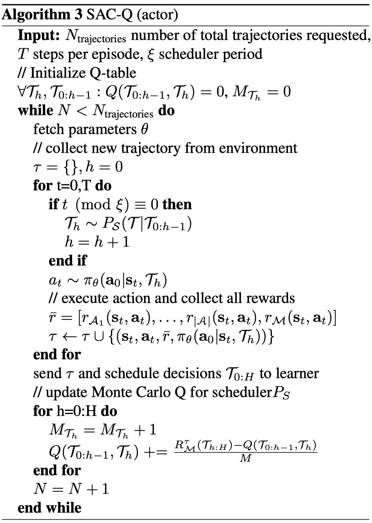
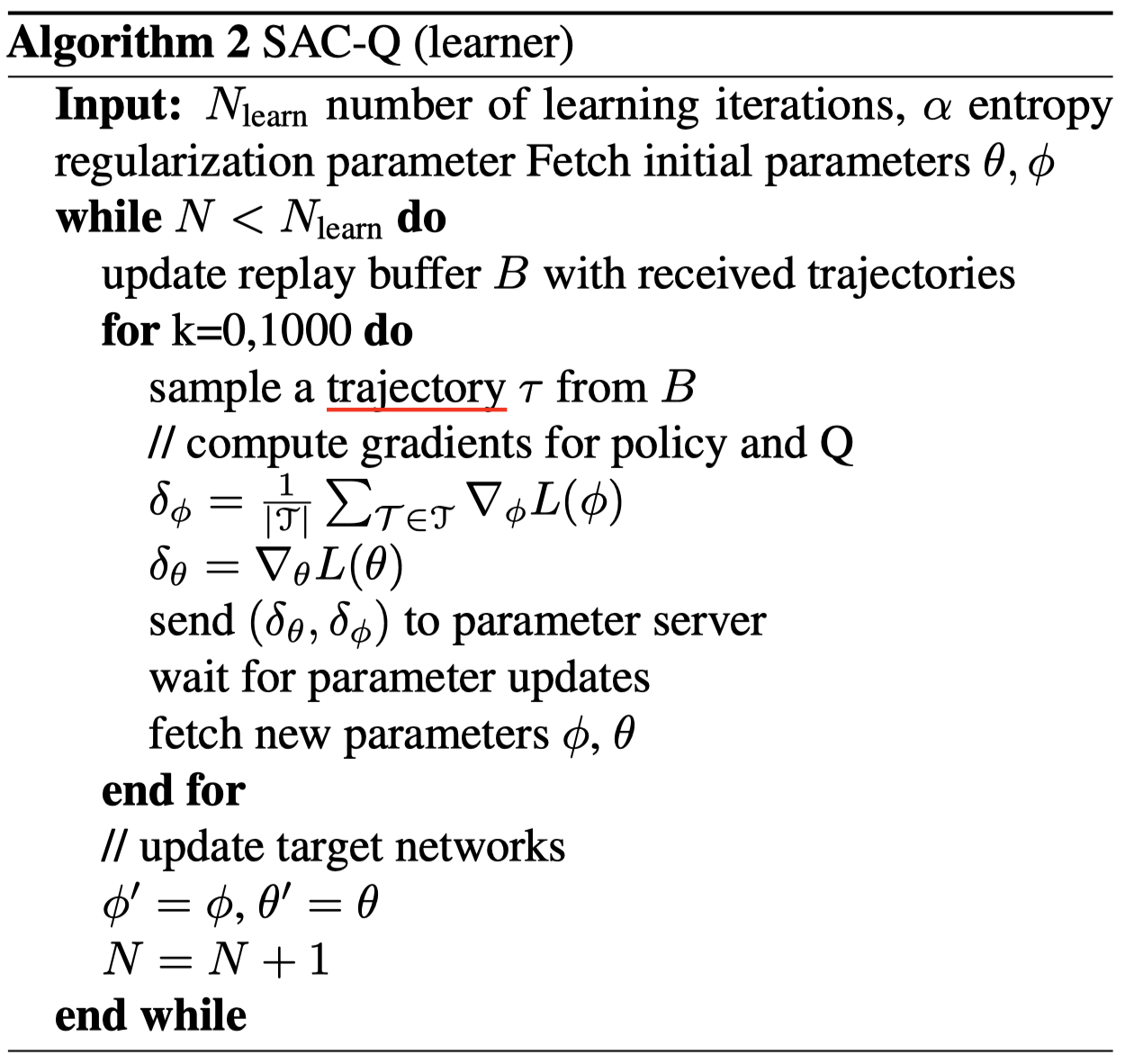
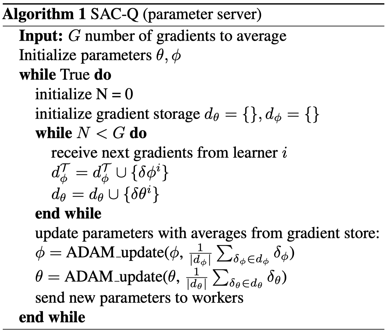
Now we present the pseudocode for the distributed SAC-X, which basically follows the architecture of Ape-X.

Actors are responsible for collecting data and update the scheduler:

Learners aggregate all collected experience inside a replay buffer, compute gradients for policy and \(Q\)-function networks, and send gradients to a central parameter server:

The parameter server update networks with gradients from the learners and handle any fetch request from the workers.

Discussion

Why not define the scheduler in terms of state?

The tabular \(Q\)-learning has the advantage of its simplicity and efficiency. Moreover, it quickly adapts to changes in the incoming stream of experience data. This is desirable for the scheduler since the intentions change over time and hence the probability that any intention triggers the main task reward is highly varying during the learning process.

The tabular \(Q\)-learning, however, is indifferent to state, which makes it more like a open-loop planning algorithm w.r.t. the environment. This may be troublesome in highly stochastic environments. As a result, I think it may be worth a trial to define the scheduler in terms of state. That is, we define the policy and \(Q\)-function as \(P_{\mathcal S}(\mathcal T\vert s)\) and \(Q(s,\mathcal T)\). The advantage of making decisions based on the state is clear: it establishes the connection between the scheduler and environment. But the deficiencies are also obvious: we now need some more sophisticated architecture to represent the \(Q\)-function, such as a neural network, which may lose the advantage of the tabular \(Q\)-learning. Furthermore, if we only use the intention for the main task at the test time, the price may not be worthy.

Some Details

The authors use ELU as activation instead of ReLU in their networks. the ELU activation is defined as

\[\begin{align} ELU(x)=\begin{cases} x,&x\ge0\\\ \alpha(e^x-1)&x<0 \end{cases} \end{align}\]

References

Martin Riedmiller et al. Learning by Playing - Solving Sparse Reward Tasks from Scratch
SAC-X code by HugoCMU
R´emi Munos et al. Safe and efﬁcient off-policy reinforcement learning