
Introduction
In reinforcement learning, planning plays a major role in model-based methods, while learning are commonly seen in model-free methods. They, however, don’t have to be separated clearly, and in fact, both shares the same paradigm: looking ahead to future events, backing up values, and then improving the policy.
In this post, we will walk though a series of planning algorithms into which learning is integrated. As stated by Sutton and Barto in their extraordinary book[1], we divide planning algorithms into two categories: background planning and decision-time planning. Background planning simulates experiences to update the value function and policy, while decision-time planning simulates experiences to select an action for a specific state. The former is preferable if low latency action selection is the priority, and the latter is most useful in applications in which fast responses are not required, such as chess playing programs.
Table of Contents
Background Planning
In background planning, the agent simulates experiences according to the learned model and uses such experiences together with real experiences to improve the value function and policy.
Dyna-Q
Our first algorithm is Dyna-Q, which focuses planning on past experiences. That is, Dyna-Q only simulates experiences for previously observed/taken \( (s, a) \), which makes it kind of similar to \( TD(\lambda) \).
Algorithm
\[\begin{align} &\mathrm{Initialize\ }Q\mathrm{\ function\ and \ }Model\\\ &\mathrm{While\ true:}\\\ &\quad \mathrm{At\ state\ }s,\ \mathrm{take\ action\ }a\mathrm{\ based\ on\ }Q\\\ &\quad\mathrm{Observe\ reward}\ r\mathrm{\ and\ state\ }s'\\\ &\quad \mathrm{Update\ }Q\ \mathrm{and\ }Model\ \mathrm{using\ transition}\ (s, a, r, s')\\\ &\quad \mathrm{Repeat}\ n\ \mathrm{times}:\quad(\mathrm{planning\ updates})\\\ &\quad\quad \mathrm{Sample\ from\ } Model\ \mathrm{transitions\ whose\ }s\ \mathrm{and\ }a\mathrm{\ are\ previously\ observed/taken}\\\ &\quad\quad \mathrm{Update\ }Q\ \mathrm{based\ on\ the\ simulated\ transitions} \end{align}\]Deficiency
Dyna-Q struggles when the model is incorrect caused by stochastic environment, defective function approximator for imperfect generalization, change of environment, etc. Especially when the environment changes to be better, Dyna-Q may not even detect such modeling error, therefore settling for a suboptimal policy.
Dyna-Q+
In some cases, the modeling error can be quickly corrected by the suboptimal policy computed by planning. That is, the model is optimistic in the sense of predicting greater reward or better state transitions than are actually possible and in doing so provides extra explorations.
Dyna-Q+ employs one such heuristic to Dyna-Q by adding extra bonus rewards to simulated experiences. In particular, if the modeled reward for a transition is \( r \), and the transition has not been tried in \( \tau \) time steps, then planning updates are done as if that transition produced a reward of \( r+\kappa\sqrt \tau \). The update rule at the planning updates now becomes
\[\begin{align} Q(s,a)=Q(s,a)+\alpha\left(r+\kappa\sqrt\tau +\gamma\max_{a'}Q(s',a')-Q(s,a)\right) \end{align}\]Another possible way is to use the extra rewards in action selection and leave the planning updates as they are in Dyna-Q. In my humble opinion, however, using the extra rewards in action selection is much short-last compared to adding the extra rewards to planning updates since \( \kappa \sqrt\tau \) immediately becomes \( 0 \) once the corresponding action is selected.
Another modification introduced by Dyna-Q+ is that it allows at the planning stage to select actions which have never been tried before. Such actions are assumed to initially lead back to the same state with a reward of zero (e.g., if \( a \) has never been tried before at state \( s \), then the modeled transition is \( (s,a, 0, s) \). The reason and effect, however, are still unclear to me — to my best knowledge, this setting may speed up the learning process by further providing some extra exploration in the early stage.
Prioritized Sweeping
Dyna agents simulate experiences started in state-action pairs selected uniformly at random from previously experienced pairs. Such an indiscriminate treatment is generally inefficient, and therefore some heuristics will come in handy.
One of such heuristics is the recency heuristic: If the value of a state changes, it is likely that the state-action pairs leading directly to that state also change, which in turn result in the changes of their predecessors, and so on. This general idea is termed backward focusing of planning computation.
Prioritized sweeping further explores the idea of backward focusing by introducing a threshold to filter out transitions which change the value function little, and prioritizing state-action pairs according to their absolute \( Q \) errors, which are referred to as priorities.
Algorithm
\[\begin{align} &\mathrm{Initialize}\ Q\ \mathrm{function\ and\ }Model\\\ &\mathrm{Initialize\ a\ priority\ queue\ } PQueue\\\ &\mathrm{Initialize\ threshold\ }\theta\\\ &\mathrm{While\ true}:\\\ &\quad \mathrm{At\ state\ }s,\ \mathrm{take\ action\ }a\mathrm{\ based\ on\ }Q\\\ &\quad\mathrm{Observe\ reward}\ r\mathrm{\ and\ state\ }s'\\\ &\quad \mathrm{Update\ }Model\ \mathrm{using\ the\ transition}\ (s, a, r, s')\\\ &\quad \mathrm{Compute\ priority\ } P(s,a)=\left|r+\max_{a'} Q(s',a')-Q(s,a)\right|\\\ &\quad \mathrm{If\ }P(s,a)>\theta\ \mathrm{ then\ insert\ }(s, a)\ \mathrm{into}\ PQueue\ \mathrm{with\ priority\ }P(s,a)\\\ &\quad \mathrm{Repeat}\ n\ \mathrm{times}:\quad(\mathrm{planning\ updates})\\\ &\quad\quad s, a=PQueue.pop()\\\ &\quad\quad \mathrm{Sample\ transition\ }(s, a, r, s')\ \mathrm{from}\ Model \\\ &\quad\quad \mathrm{Update\ }Q\ \mathrm{using\ transition\ }(s,a,r,s')\\\ &\quad\quad \mathrm{For\ all\ }s^-, a^-\ \mathrm{predicted\ to\ lead\ to}\ s:\\\ &\quad\quad\quad r^-=\mathrm{predicted\ reward\ for\ }(s^-,a^-,s)\\\ &\quad\quad\quad P(s^-,a^-)=\left|r^-+\max_{a}Q(s,a)-Q(s^-, a^-)\right|\\\ &\quad\quad\quad \mathrm{If\ }P(s^-,a^-)>\theta\ \mathrm{ then\ insert\ }(s^-, a^-)\ \mathrm{into}\ PQueue\ \mathrm{with\ priority\ }P(s^-,a^-) \end{align}\]Trajectory Sampling
Trajectory sampling simulates trajectories according to the model learned when following the current policy. It is on-policy since the policy it follows to interact with the model is the same policy it employs to interact with the environment. This helps to speed up the learning process but may impair the ultimate performance in the long run. Both of these make sense. Trajectory sampling according to the on-policy distribution puts more considerations on those states frequently visited when following the current policy and ignores vast uninteresting states. In the short run, such focusing helps the learning process concentrate on what’s most relevant (and promising if the policy is kind of greedy). In the long run, the lack of exploration may result in the algorithm settling for a sub-optimal performance. As a result, trajectory sampling gains a great advantage for large problems, in particular for problems in which only a small subset of the state-action space is visited under the policy.
Algorithm
\[\begin{align} &\mathrm{Initialize\ }Q\mathrm{\ function\ and \ }Model\\\ &\mathrm{While\ true:}\\\ &\quad \mathrm{At\ state\ }s,\ \mathrm{take\ action\ }a\mathrm{\ based\ on\ }Q\\\ &\quad \mathrm{Observe\ reward}\ r\mathrm{\ and\ state\ }s'\\\ &\quad \mathrm{Update\ }Q\ \mathrm{and\ }Model\ \mathrm{using\ transition}\ (s, a, r, s')\\\ &\quad \mathrm{Repeat}\ n\ \mathrm{times}:\quad(\mathrm{planning\ updates})\\\ &\quad\quad \mathrm{Sample\ from\ } Model\ \mathrm{transitions\ }, (s, a, r, s'), \mathrm{\ starting\ from\ state\ }s\ \mathrm{and\ action\ }a\\\ &\quad\quad \mathrm{Update\ }Q\ \mathrm{based\ on\ the\ simulated\ transitions}\\\ &\quad\quad \mathrm{Select\ action\ }a'\ \mathrm{based\ on\ the\ current\ policy}\\\ &\quad\quad s, a=s', a' \end{align}\]Real-Time Dynamic Programming
Value iteration is a dynamic programming algorithm based on the Bellman optimality equation
\[\begin{align} V(s)=\max_{a}\sum_{s',r}p(s', r|s, a)(r+\gamma V(s')) \end{align}\]In the vanilla value iteration, it applies the Bellman optimality equation to all states at every iteration until the value function converges. This is, however, not necessary. Asynchronous dynamic programming algorithms update state values in any order whatsoever, using whatever values of other states happen to be available. Real-Time Dynamic Programming(RTDP) is an example of asynchronous dynamic programming algorithms, in which we only update states that are relevant to the agent at the current timestamp (e.g. the current state and states visited in limited-horizon look-ahead search from the current state).
Algorithm
\[\begin{align} &\mathrm{For\ each\ step\ in\ a\ real\ or\ simulated\ trajectory}:\\\ &\quad s=\mathrm{current\ state}\\\ &\quad\mathrm{Take\ a\ greedy\ action\ }a\\\ &\quad V(s)=\sum_{s', r}p(s',r|s, a)(r+\gamma V(s'))\\\ &\quad \mathrm{While\ time\ remains,\ for\ each\ successor\ state\ }s':\\\ &\quad\quad V(s') = \max_{a'}\sum_{s'', r'}p(s'', r'|s', a')(r'+\gamma V(s'')) \end{align}\]Convergence
For problems, with each episode beginning in a state randomly chosen from the set of start states and ending at a goal state, RTDP converges with probability one to a policy that is optimal for all the relevant states provided:
- The initial value of every goal state is zero.
- There exists at least one policy that guarantees a goal state will be reached with probability one from any start state.
- All rewards for transitions from non-goal states are strictly negative.
- All the initial values are equal to, or greater than, their optimal values (i.e., optimistic initial value, which can be satisfied by simply setting the initial values of all states to zero).
Conditions 3 and 4 requires the initial values are admissible and consistent, which guarantees sufficient exploration.
Tasks having these properties are examples of stochastic optimal path problem, which are usually stated in terms of cost minimization instead of reward maximization.
In fact, RTDP could be reduced to a heuristic online search algorithm, namely Learning Real-Time A*(LRTA*), if all transitions are deterministic.
Advantages
There are some advantages of RTDP:
- RTDP is guaranteed to find an optimal policy on the relevant states without visiting every state infinitely often, or even without visiting some states at all. This could be a great advantage for problems with very large state sets, where even a single sweep may not be feasible
- The conventional DP algorithm could produce a greedy policy that is optimal long before it converges. Checking for the emergence of an optimal policy before value iteration converges requires considerable additional computation. The greedy policy used by RTDP to generate trajectories, on the other hand, approaches the optimal policy as the value function approaches to the optimal value function, so there is no need for an additional check for the emergence of an optimal policy in RTDP.
Decision-Time Planning
In decision-time planning, the agent focuses on a particular state and uses simulated trajectories to select an action for that state. The key idea here is forward search and sampling — the agent only considers states from the current state onward and relies on simulation to make decision.
Rollout Algorithms
Rollout algorithms estimate action values by averaging the returns of many simulated trajectories that start with each possible action and then follow the given rollout policy.
Because a rollout algorithm takes the best action on the current state evaluated in terms of the rollout policy — in another word, it differs from the rollout policy only at the current state — the resultant policy should be at least as good as, or better than the rollout policy. This brings us the intuition that the better the rollout policy and the more accurate the value estimates, the better the policy produced by a rollout algorithm is likely to be.
Computational Considerations
As decision-time planning methods, rollout algorithms usually have to meet strict time constraints. The computation time needed by a rollout algorithm depends on:
- The number of actions that have to be evaluated for each decision.
- The number of time steps in the simulated trajectories needed to obtain useful sample returns.
- The time it takes the rollout policy to make a decision
- The number of simulated trajectories needed to obtain good Monte Carlo action-value estimates.
There are several ways to ease the computational requirements:
- Since the trajectories are simulated independent of one another, it is possible to run many trials in parallel on separate processors.
- It may not be necessary to simulate the entire trajectory, the \( n \)-step return will come in handy if the value function is computed during the process.
- It is also possible to monitor the simulations and prune away candidate actions that are unlikely to turn out to be the best, or whose values are close enough to that of the current best that choosing them instead would make no real difference (though Tesauro and Galperin(1997) point out that this would complicate a parallel implementation).
Monte Carlo Tree Search
Monte Carlo Tree Search(MCTS) is a rollout algorithm, which introduces an accumulative tree to direct simulations towards more highly-rewarding trajectories.
Terminnologies
Before diving into the details of MCTS, we first introduce some terminologies which will be used later.
Nodes in The Tree
In the accumulative tree, nodes are divided into two parts:
- Non-leaf nodes, on which we perform tree policy. Non-leaf nodes are fully expanded — there should not be any unexplored action from it.
- Leaf nodes, from which we expand the tree and run simulation. There should be some actions from the leaf nodes left to explore.
It’s important to be aware that Leaf nodes does not refer to an unexplored node. If we take an unexplored node as leaf, this could incur additional \(O(N)\) memory complexity, where \(N\) is the number of leaf nodes in the tree.
Policies
There are two different policies playing in MCTS:
- Tree policy, which is used to pick actions within the tree. A tree policy could be any policy that takes into account both exploration and exploitation, a typical choice is Upper Confidence Bound
where the first term computes the expected state-action value and the second term measures the uncertainty or variance in the estimates of the state-action value.
- Rollout policy, which simulations or rollouts are performed based on. A rollout policy may simply be a uniform random policy.
Algorithm
Following steps describes what is going on at each state:
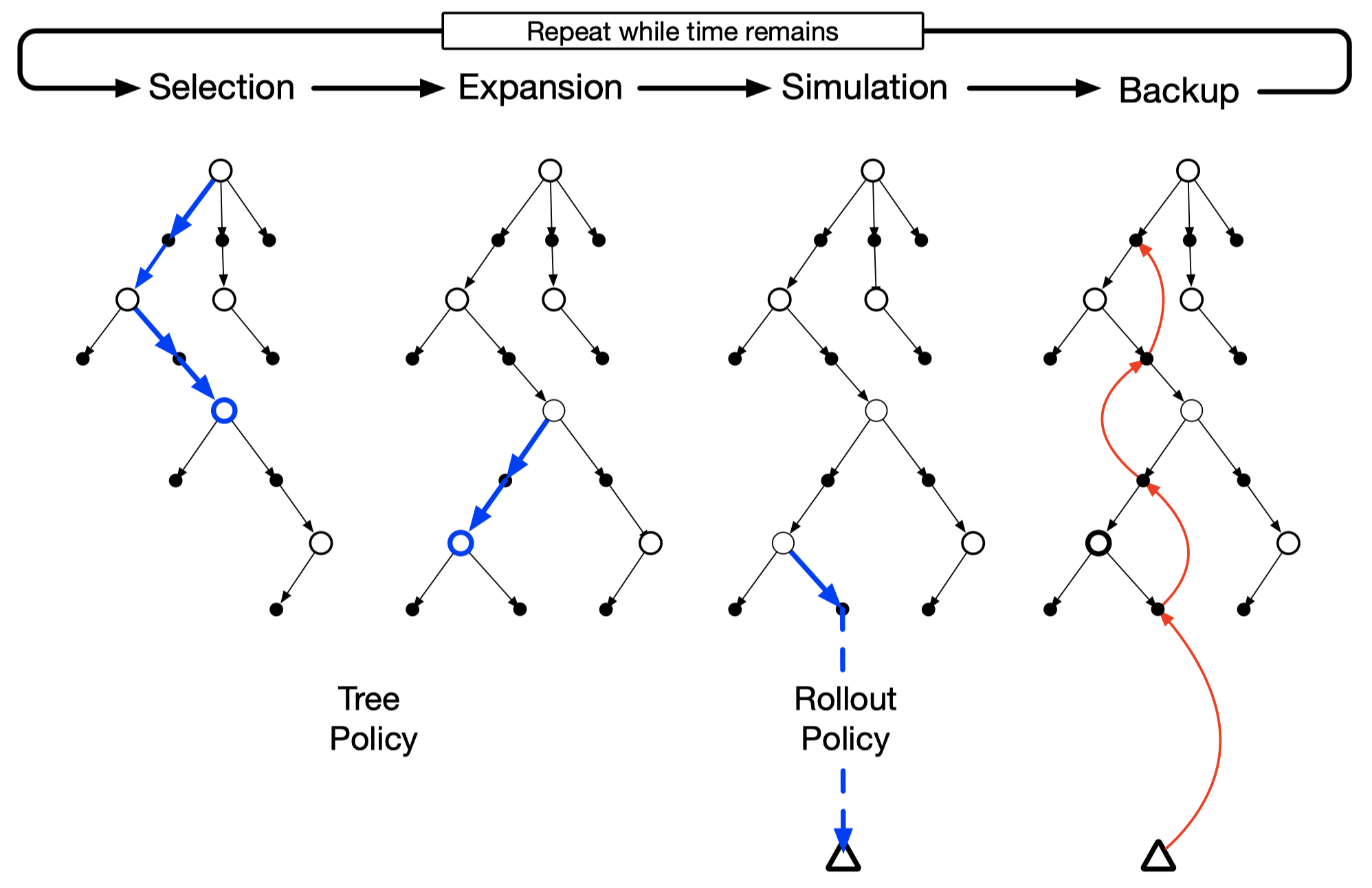
- Selection: Perform the tree policy from the root traversing down to a leaf node
- Expansion: Expand the tree from the selected leaf node by adding one or more child nodes reached from the selected leaf node via unexplored actions
- Simulation: Run a simulation according to the rollout policy from one of the newly-added children
- Backpropagation: Back propagate the simulation results to the root. Only values of nodes in the tree get updated/saved. No values are saved for the states and actions beyond the tree.
The above four steps repeat until no more time is left, or some other computational resource is exhausted. Then finally, an action from the root node is selected to take according to some mechanism that depends on the accumulated statistics in the tree; for example, it may be an action having the largest action value, or perhaps the action with the largest visit count to avoid selecting outliners.
After the environment transitions to a new state, the above process is run again, starting with a tree containing any descendants of this node left over from the tree constructed by the previous execution of MCTS, all remaining nodes are discarded, along with the action values associated with them.
TD Search
As we mentioned at the beginning of decision-time planning, the key idea here is forward search and sampling. Therefore, there is no strict need for running a whole episode to the end of the game.
TD Search differs from MCTS only in that TD Search bootstraps the action-value function and uses SARSA to update the action-value function. In this way it gains advantages of TD methods and outperforms MCTS especially in Markov environments.
Dyna-2
Dyna-2 integrates TD search with TD learning, in which there are two categories of memory:
- long-term memory: general domain knowledge that applies to any episode
- short-term memory: specific local knowledge about the current situation
The long-term memory is updated from real experience using TD learning, while the short-term memory is updated from simulated experience via TD search.
At last, we sum up the long- and short-term memories to help with action selection at the current state.