
Table of Contents
Generative Query Network
Introduction
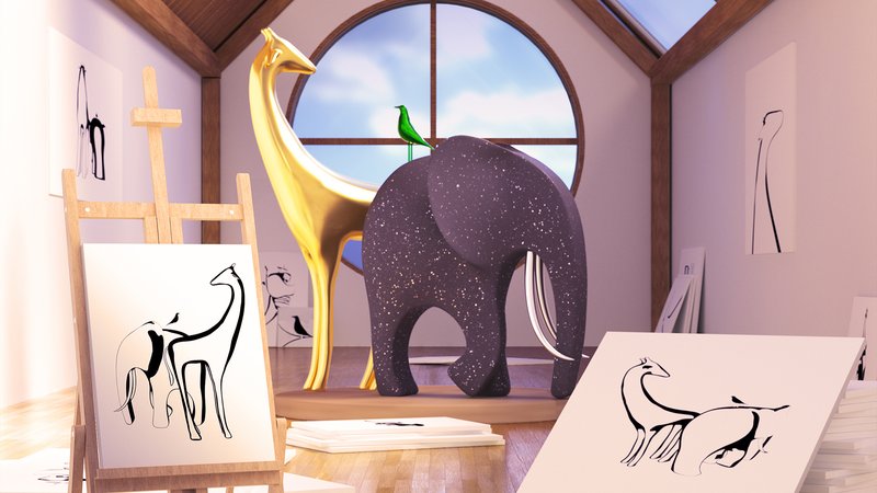
The generative query network(GQN) is an unsupervised generative network, published on Science in July 2018. It’s a scene-based method, which allows the agent to infer the image from a viewpoint based on the pre-knowledge of the environment and some other viewpoints. Thanks to its unsupervised attribute, the GQN paves the way towards machines that autonomously learn to understand the world around them.
In a nutshell, the GQN is mainly comprised of three architectures: a representation, a generation, and an auxiliary inference architecture. The representation architecture takes images from different viewpoints to yield a concise abstract scene representation whereby the generation architecture sequentially generates an image for a new query viewpoint. The inference architecture serving as the encoder in a variational autoencoder provides a way to train the other two architectures in an unsupervised manner.
Now let’s delve into these three architectures and see what they look like.
Representation Architecture
The representation architecture describes the true layout of the scene by capturing the most important elements, such as object positions, colors and room layout, in a concise distributed representation
Input & Output
Input: For each scene \( i \), the input is comprised of observed images \( \mathbf x_i^{1,\dots,M} \) and their respective viewpoints \( \mathbf v_i^{1, \dots, M} \), where the superscript indicates different recorded views for a scene. Each viewpoint \( \mathbf v_i^k \) is parameterized by a 7-dimensional vector
\[\begin{align} \mathbf v^k = \left(\mathbf w, \cos(\mathbf y^k), \sin(\mathbf y^k), \cos(\mathbf p^k), \sin(\mathbf p^k) \right) \end{align}\]where \( \mathbf w \) consists of the 3-dimensional position of the camera, and \( \mathbf y \) and \( \mathbf p \) correspond to its yaw and pitch respectively.
Output: Representation \( \mathbf r \), an effective summary of the observations at a scene, computed by the scene representation network:
\[\begin{align} \mathbf r^k&=\psi(\mathbf x^k, \mathbf v^k)\\\ \mathbf r &= \sum_{k=1}^M \mathbf r^k \end{align}\]where \( \psi \) is a ConvNet shown next, and \( \mathbf r \) simply the element-wise sum of all \( \mathbf r^k \).
Candidate Networks
The authors experiment three different architectures:
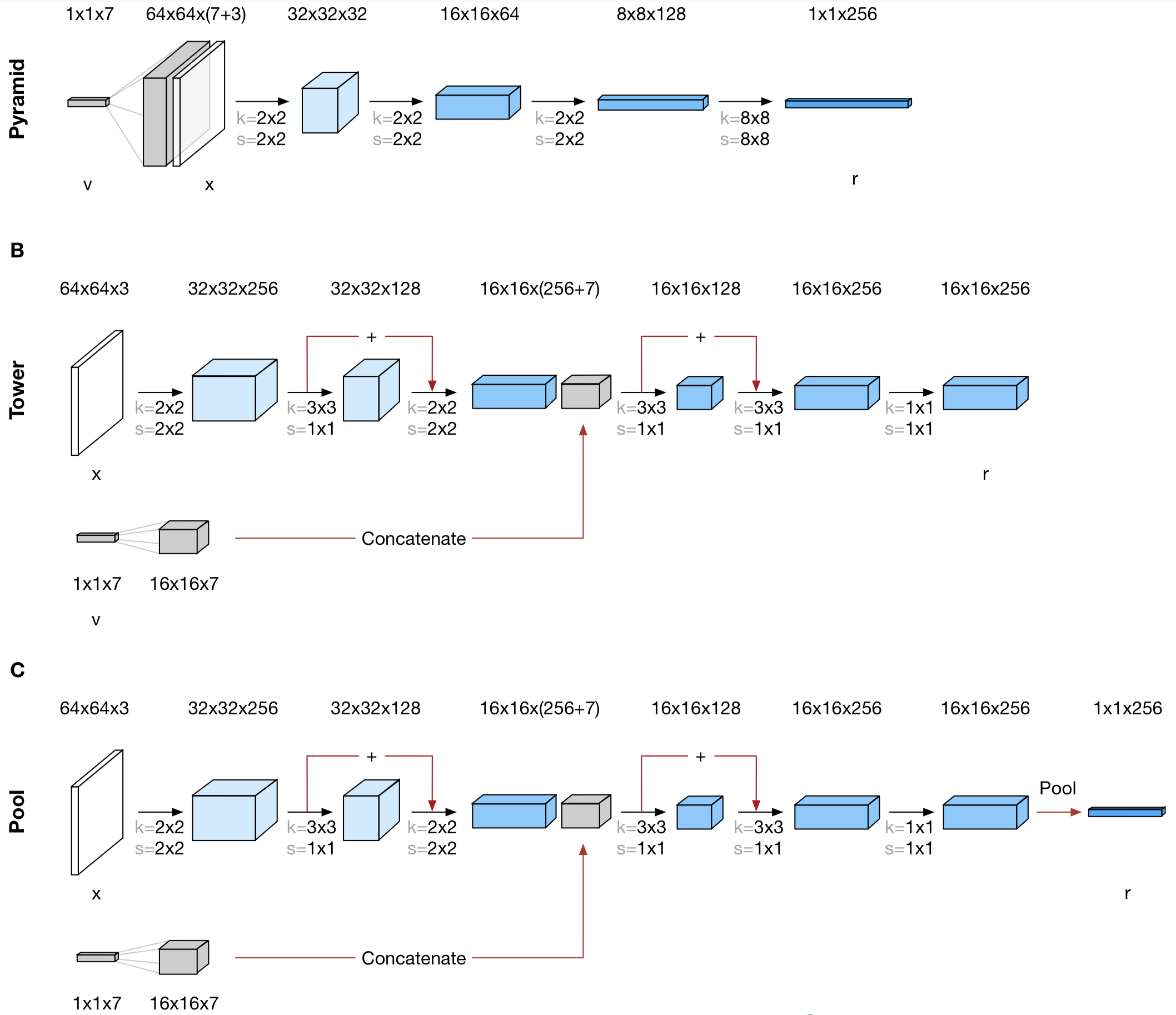
<a name=”back1’></a>They find the ‘Tower’ architecture to learn fastest across datasets and to extrapolate quite well. And interestingly, these three architectures do not have the same factorization and compositionality properties. I”ll leave the discussions of the properties of the scene representation in the end.
Generation Architecture
During training, the generator learns about typical objects, features, relationships, and regularities in the environment. This shared set of ‘concepts’ enables the representation network to describe the scene in a highly compressed, abstract manner, leaving it to the generation network to fill in the details where necessary.
Input & Output
Input: Query viewpoint \( \mathbf v^q \), representation \( \mathbf r \) for a set of \( \mathbf x \) and \( \mathbf v \) at the same scene as the query viewpoint, latent variable vector \( \mathbf z \)
Output: Query image \( \mathbf x \) corresponding to \( \mathbf v^q \).
Network
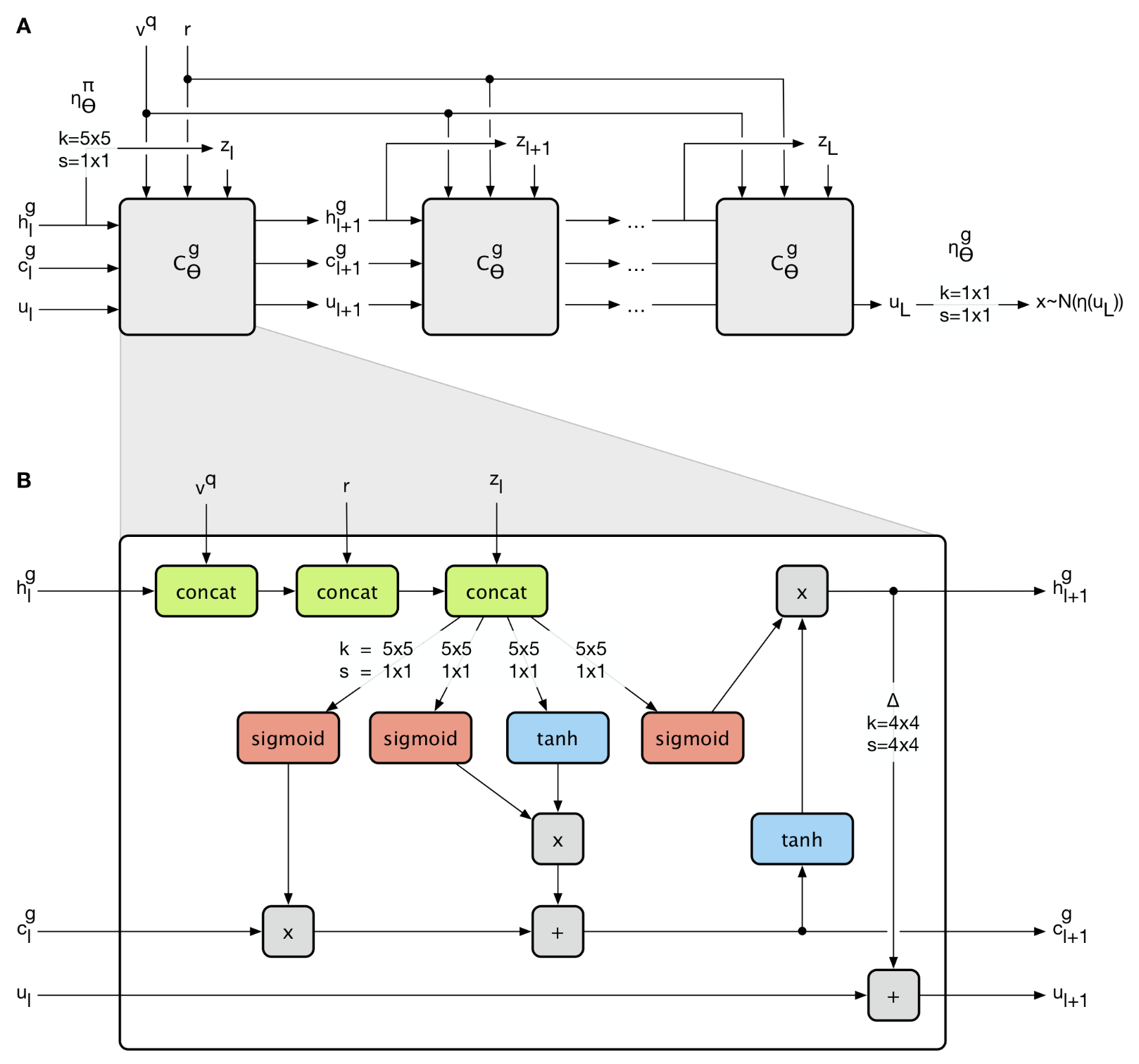
The query viewpoint \( \mathbf v^q \) and the representation \( \mathbf r \) are the same across LSTM cells, while the latent vector \( \mathbf z_l \) is derived from the hidden state \( h_l^g \), which means it varies depending on \( h_l^g \). Moreover, \( \mathbf z_l \) is sampled from the prior \( \pi_{\theta}(\mathbf z_l\vert \mathbf v^q,\mathbf r, \mathbf z_{< l})=\mathcal N (\mathbf z_l\vert \eta_{\theta}^\pi( h_l^g)) \), a Gaussian distribution whose mean and standard deviation are computed from the ConvNet \( \eta_\theta^\pi(h_l^g) \). (In the draft I read, the authors parameterize \( \pi \) with \( \theta_l \), i.e. using \( \pi_{\theta_l} \) instead of \( \pi_\theta \) in the left hand of the equation. they explain that \( \theta_l \) refers to the subset of parameters \( \theta \) that are used by the conditional density at step \( l \). However, in my humble opition, LSTM cell shares the same weights over timestamps, which makes this subset concept redundant)
This recurrent architecture splits the vector of latent variables \( \mathbf z \) into \( L \) groups of latent \( \mathbf z_l \), \( l=1, \dots, L \), due to which the prior \( \pi_\theta(\mathbf z\vert \mathbf v^q, \mathbf r) \) can be written as an auto-regressive density:
\[\begin{align} \pi_\theta(\mathbf z|\mathbf v^q, \mathbf r) = \prod_{l=1}^L\pi_\theta(\mathbf z_l|\mathbf v^q, \mathbf r, \mathbf z_{< l}) \end{align}\]The generated image is sampled from the generator \( g_{\theta}(\mathbf x^q\vert \mathbf z, \mathbf v^q,\mathbf r) = \mathcal N (\mathbf x^q\vert \mu=\eta_\theta^g(\mathbf u_L), \sigma=\sigma_t) \), also a Gaussian distribution, whose mean is computed from the ConvNet \( \eta_\theta^g(u_l) \), and standard deviation is annealing towards \( 0.7 \) over the duration of training. The authors explain that annealing variance encourages the model to focus on large-scale aspects of the prediction problem in the beginning and only later on the low-level details
The workflow at each skip-connection convolutional LSTM cell is given as below:
- Concatenate \( \mathbf v^q,\mathbf r, \mathbf z_l \) to hidden state \( \mathbf h_l^g \)
- Pass the resulting tensor to convolutional layers with sigmoid/tanh as activations to compute forget gate, input gate, candidate values and output gate separately
- As in general LSTM, update cell state and hidden state sequentially
- Upsample the hidden state via transposed convolutional layer and add the result to \( \mathbf u_l \). Notice that \( u_l \) is constructed bit by bit as LSTM unrolls. This indicates that our eventual image is also constructed part by part as time goes by.
Inference Architecture
The inference architecture acts much like the encoder network in VAE, which is mainly used to approximate the latent variable distribution, thereby training the other two architectures.
Input: Representation \( \mathbf r \), query viewpoint \( \mathbf v^q \), query image \( \mathbf x^q \)
Output: The variational posterior density \( q_\phi(\mathbf z\vert \mathbf x^q,\mathbf v^q,\mathbf r) \), a Gaussian treated as the approximation to \( \pi_\theta(\mathbf z\vert \mathbf v^q, \mathbf r) \).
Network
Unfortunately the inference network \( C_\phi^e \) is not mentioned in the draft I read, I boldly try to draw it myself based following evidence I extract from the draft:
- Unlike the generation network \( C_\theta^g \), it takes \( \mathbf x^q \) rather than \( \mathbf z \) as one of its inputs
- \( \theta \) is a subset of \( \phi \)
- It somehow depends on \( h_l^g \), the hidden state of the \( C_\theta^g \)
- It doesn’t update \( \mathbf u_l \)
- Inference network works in parallel with the generation network to compute the loss function
Here’s the LSTM cell for inference architecture I draw
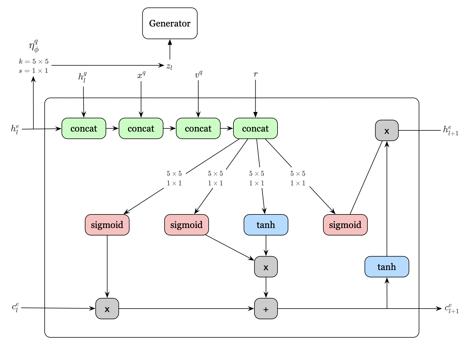
The workflow shares most similarity with the generation architecture, except that now there is no \( \mathbf u \) to update and the inference architecture produces as output the variational posterior density \( q_\phi(\mathbf z\vert \mathbf x^q,\mathbf v^q,\mathbf r) \).
Inference Architecture with Reinforcement Learning
In my humble option, the inference architecture may be able to cooperate with reinforcement learning algorithms, by adding another downstream just as \( \mathbf u \) in the generation architecture. It is more like a food for thought, still requiring further studies.
Optimization
The loss function is derived almost the same as the variational autoencoder except that now we want to maximize the conditional probability \( p_\theta(\mathbf x\vert \mathbf v^q, \mathbf r) \). For a detailed derivation, please refer to my previous post for VAE. Here we just deliver the ultimate loss function
\[\begin{align} \mathcal L(\theta, \phi) = E_{(\mathbf x, \mathbf v)\sim D, z\sim q_\phi}\left[-log\mathcal N(x^q|\eta_\theta^g(\mathbf u_L)) + \sum_{l=1}^L D_{KL}[\mathcal N(\mathbf z|\eta_\phi^q(\mathbf h_l^e))\Vert\mathcal N(\mathbf z|\eta_\theta^\pi(\mathbf h_l^g))] \right] \end{align}\]The Loss function mainly consists of two parts:
- Reconstruction likelihood: \( -log\mathcal N(x^q\vert \eta_\theta^g(\mathbf u_L)) \). This term measures how likely the image produced by the generator is to the real query image. It is crucial to realize that the latent variable \( z \) is sampled from \( q_\phi \), not from \( \eta^\pi_\theta \). This makes sense why we anticipate the generator to generate the query image \(\mathbf x^q \). Also because of that, the reconstruction likelihood does not involve the update of the ConvNet \( \eta^\pi_\theta \).
- The KL divergence of the posterior approximate \( q_\phi(\mathbf z_l\vert \mathbf x^q, \mathbf v^q, \mathbf r, \mathbf z_{< l}) \) from the prior \( \pi_\theta(\mathbf z_l\vert \mathbf v^q,\mathbf r, \mathbf z_{< l}) \). This term penalizes the difference between the distribution of the latent variable \( \mathbf z \) used in the generator and that in the inference architecture. Note that this term is measured sequentially in the network and can be calculated analytically by conditioning on the previous latent sample. A detailed analytical computation of the KL divergence between two Gaussians will be appended in the end. Another thing worth some attention is that, as the reconstruction likelihood disregards the prior \( \pi_\theta(\mathbf z\vert \mathbf v^q,\mathbf r) \), the KL divergence does not contribute to the update of the transpose convolutional layer in \( C_\theta^g \)
Algorithm Pseudocode
Loss
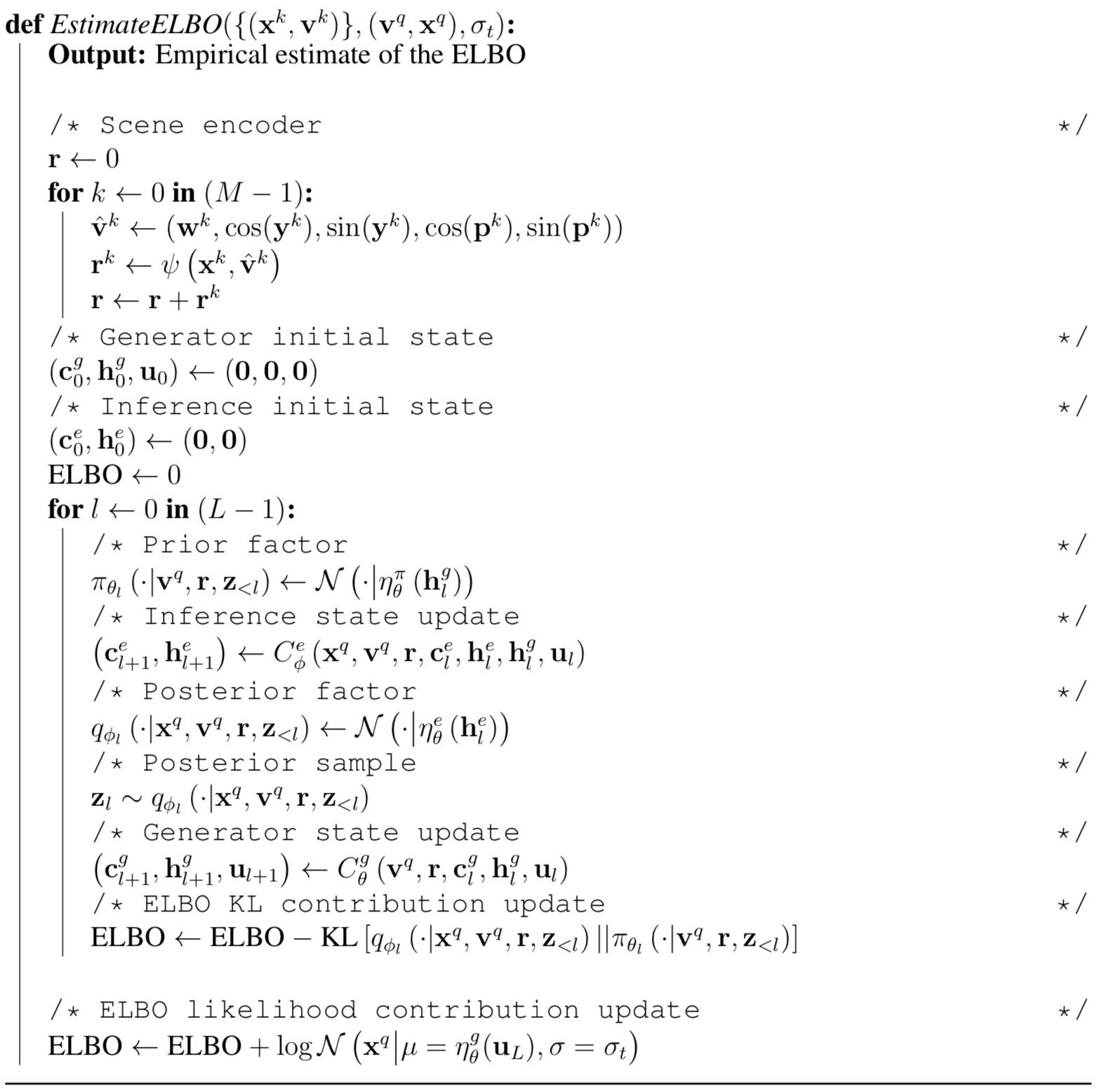
To compute the ELBO, we first construct the representation \( \mathbf r \), then we run the generator architecture in parallel with the inference architecture, computing the KL divergence sequentially. At last, we add the reconstruction likelihood to form the ELBO.
Training
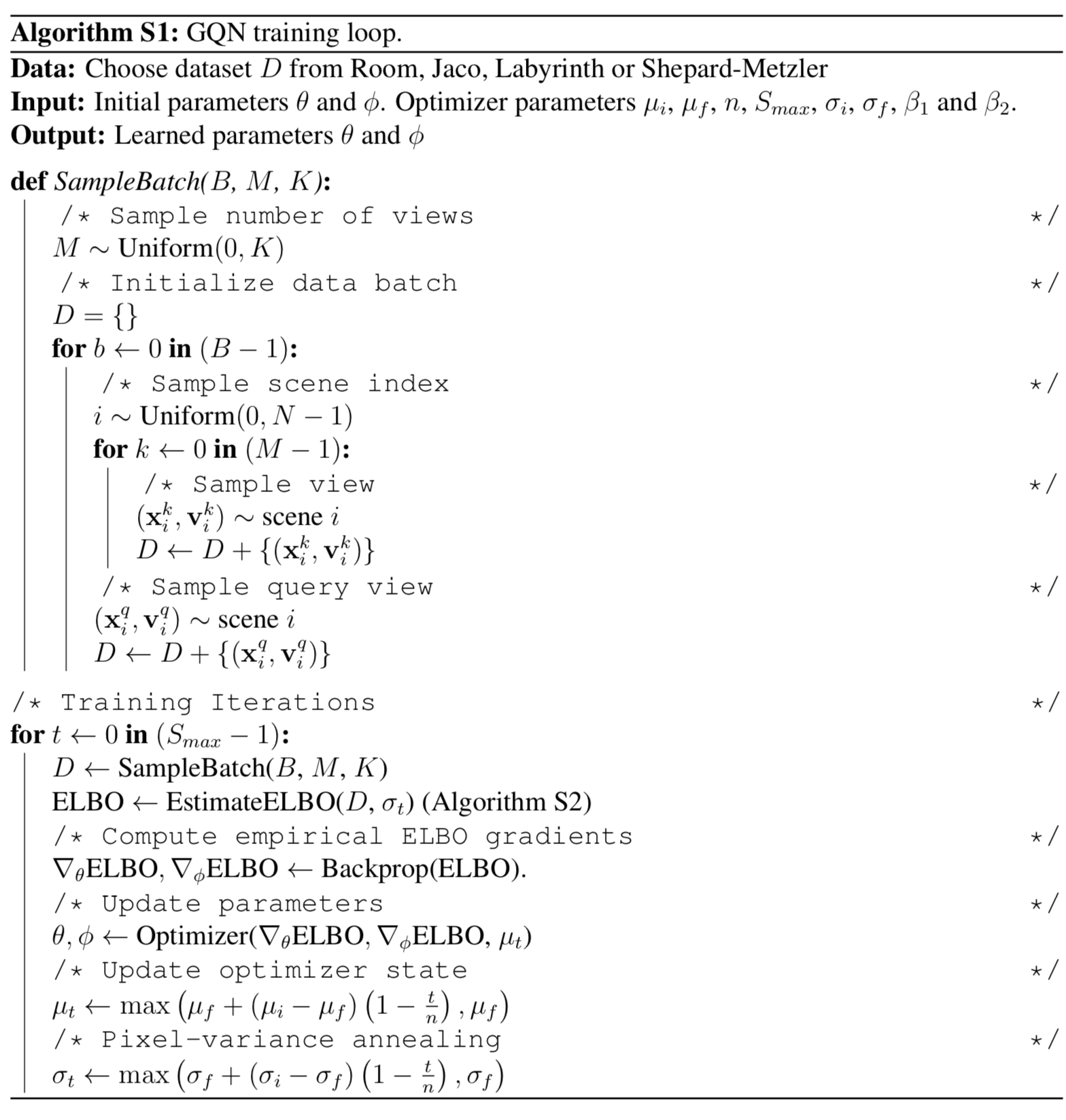
At each training step, we first choose a batch of scene points. For each scene, we sample several viewpoints and their corresponding images, along with the query viewpoint and image to form our training data. Then we compute the loss function and optimize our network using Adam optimizer.
Generation
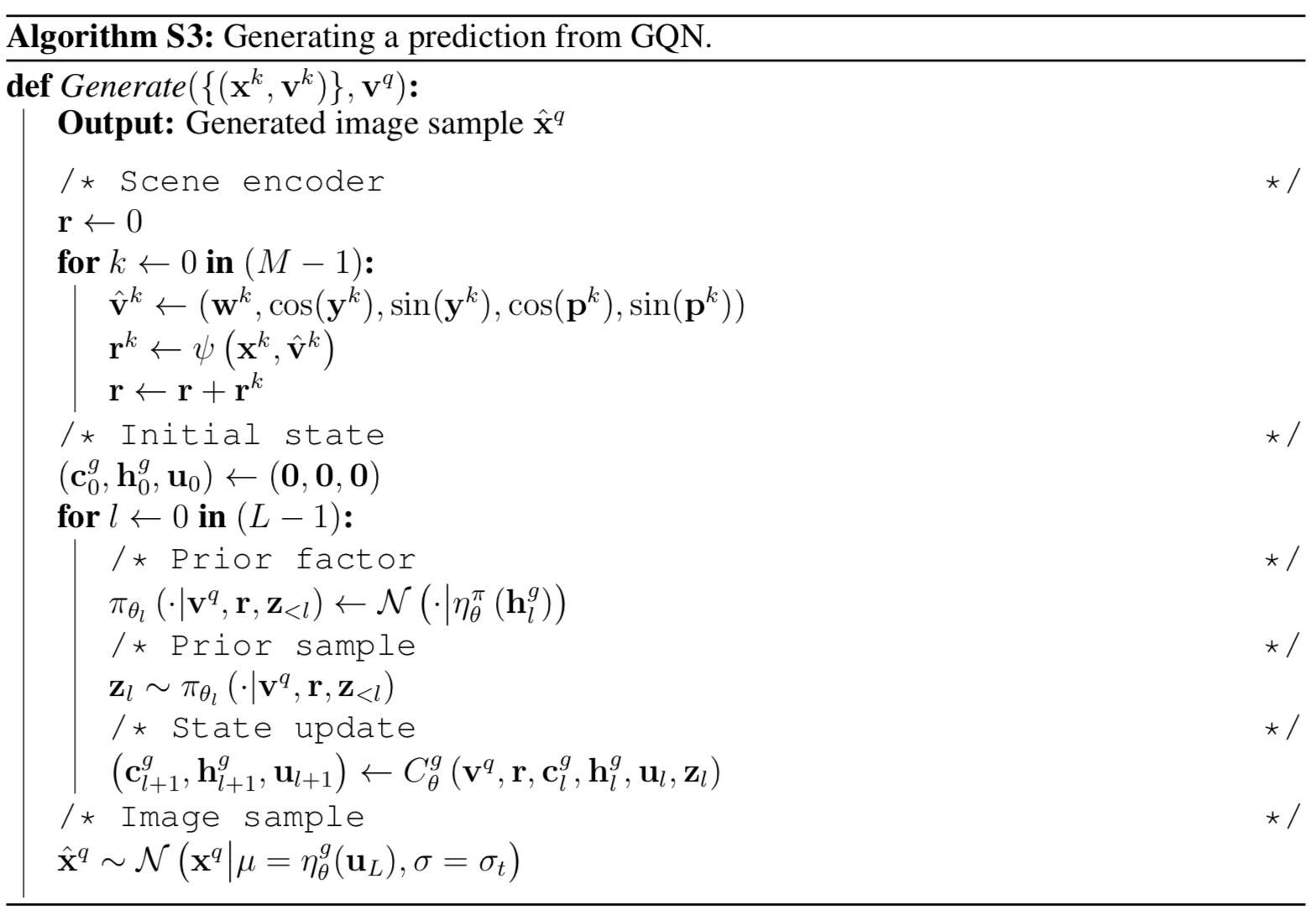
At generation stage, we first compute the representation at the query scene and then run through the generation network to compute a Gaussian distribution from which we sample our query image.
Supplementary Materials
Properties of The Scene Representation
The abstract scene representation exhibits some desirable properties as follows:
- T-SNE visualization of GQN scene representation vectors shows clear clustering of images of the same scene despite remarkable changes in viewpoint
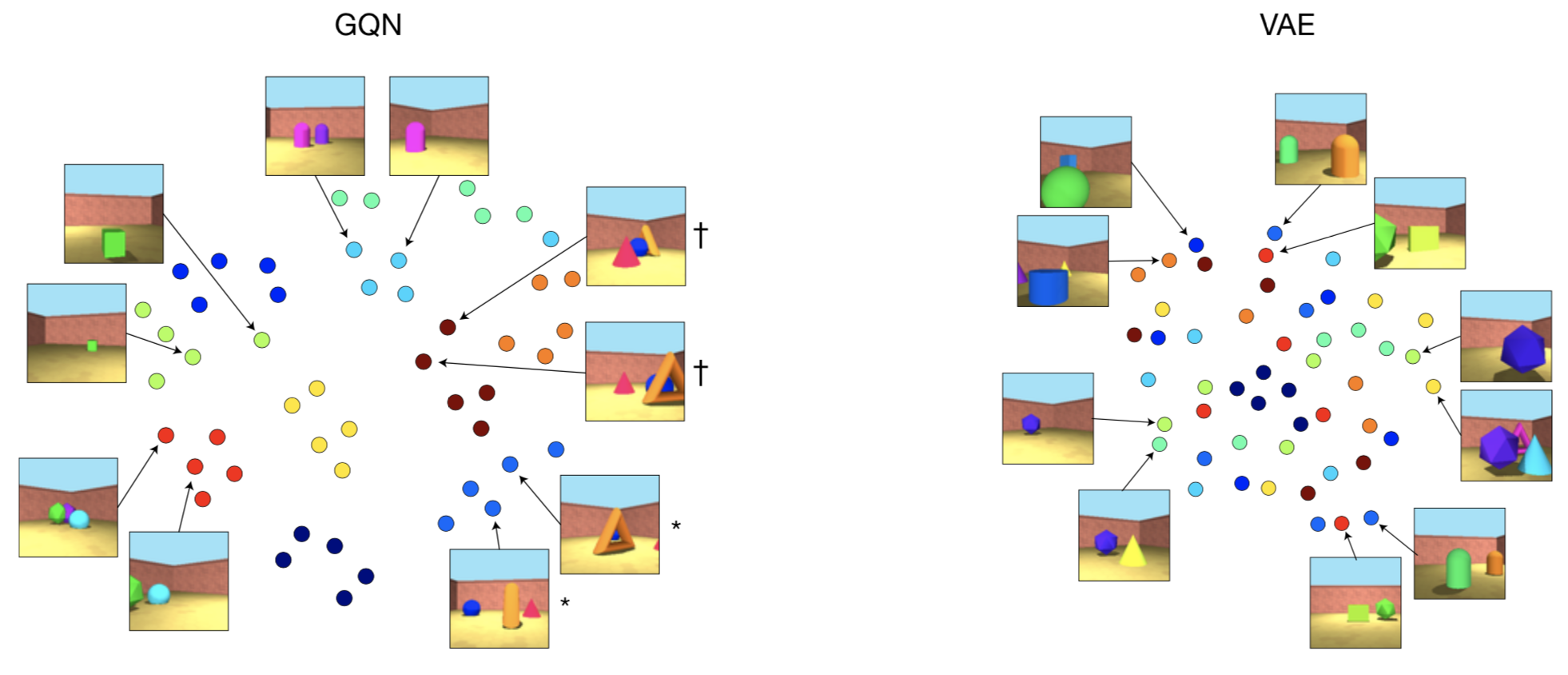
</figure>
- When prompted to reconstruct a target image, GQN exhibits compositional behavior as it is capable of both representing and rendering combinations of scene elements it has never encountered during training. An example of compositionality is given below
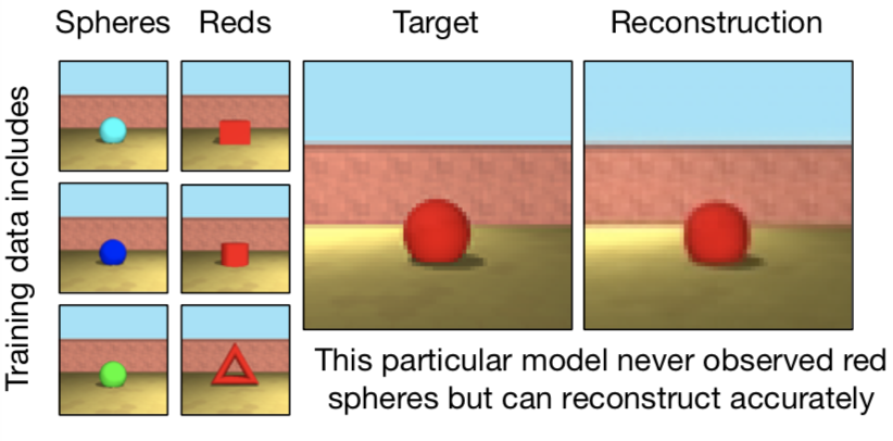
</figure>
- Scene properties, such as object color, shape, size, etc. are factorized — change in one still results in a similar representation
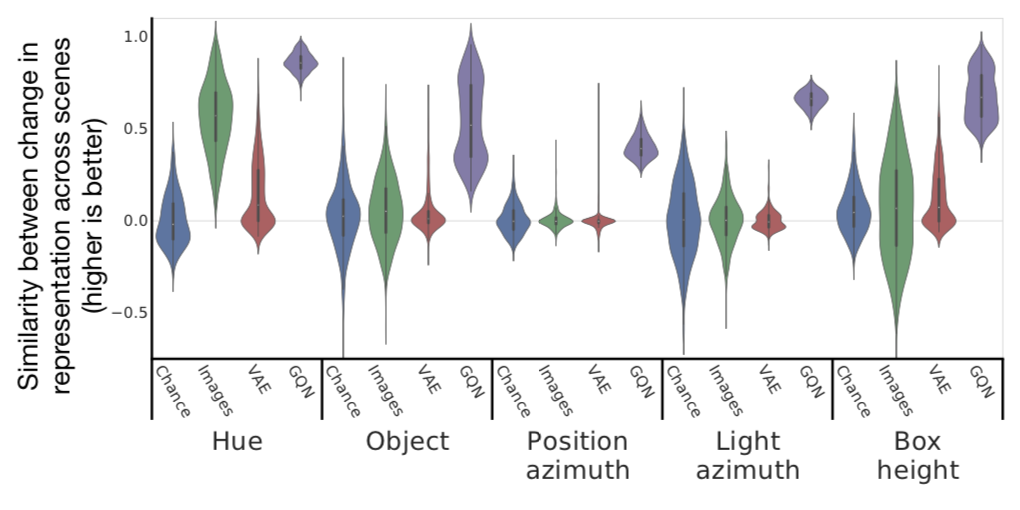
</figure>
- GQN is able to carry out scene algebra. That is, by adding and subtracting representations of related scenes, object and scene properties can be controlled, even across object positions
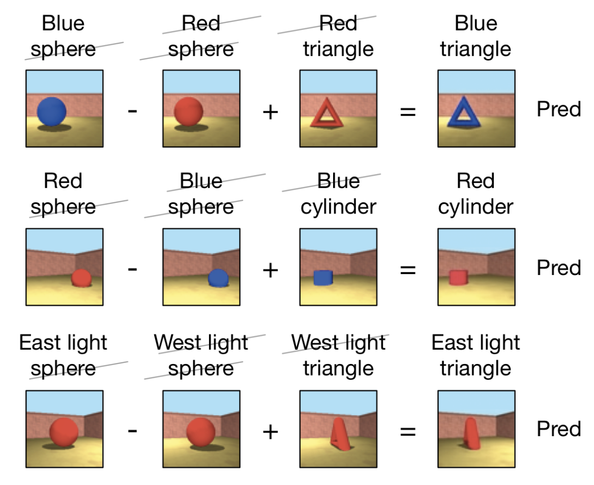
</figure>
- Because it’s a probabilistic model, GQN also learns to integrate information from different viewpoints in an efficient and consistent manner. That is, the more viewpoints are provided, the more accurate the prediction is likely to be.
Analytical Computation of The KL Divergence Between Two Gaussians
\[\begin{align} q(x)=\mathcal N(x;\mu_1, \sigma_1)\\\p(x)=\mathcal N(x;\mu_2, \sigma_2) \end{align}\]Assuming we have two Gaussians: \( q(x)=\mathcal N(x;\mu_1, \sigma_1), p(x)=\mathcal N(x;\mu_2, \sigma_2) \), now we compute their KL divergence \( D_{KL}\left(q(x)\Vert p(x)\right)=E_q\left[\log q(x)-\log p(x)\right] \) as follows
\[\begin{align} D_{KL}\left(q(x)\Vert p(x)\right)&=E_q\left[\log q(x)-\log p(x)\right]\\\ &=E_q\left[-{1\over 2}\log(2\pi)-\log \sigma_1-{1\over 2}\left(x-\mu_1\over \sigma_1\right)^2+{1\over 2}\log(2\pi)+\log \sigma_2+{1\over 2}\left(x-\mu_2\over \sigma_2\right)^2\right]\\\ &=\log{\sigma_2\over \sigma_1}+{1\over 2\sigma_2^2}E_q\left[\left(x-\mu_2\right)^2\right]-{1\over 2\sigma_1^2}E_q\left[\left(x-\mu_1\right)^2\right]\\\ &=\log {\sigma_2\over \sigma_1}+{1\over 2\sigma_2^2}E_q\left[\left(x-\mu_1+\mu_1-\mu_2\right)^2\right]-{1\over 2}\\\ &=\log {\sigma_2\over \sigma_1}+{1\over 2\sigma_2^2}E_q\left[\left(x-\mu_1\right)^2+2\left(x-\mu_1\right)\left(\mu_1-\mu_2\right)+\left(\mu_1-\mu_2\right)^2\right]-{1\over 2}\\\ &=\log {\sigma_2\over \sigma_1}+{1\over 2\sigma_2^2}\left(\sigma_1^2 +0+\left(\mu_1-\mu_2\right)^2\right)-{1\over 2}\\\ &=\log{\sigma_2\over \sigma_1}+{\sigma_1^2+\left(\mu_1-\mu_2\right)^2\over 2\sigma_2^2}-{1\over 2} \end{align}\]For multivariate Gaussians with a diagonal covariance matrix, let \( J \) be the dimensionality of \( \mathbf x \), we’ll have
\[\begin{align} D_{KL}\left(q(\mathbf x)\Vert p(\mathbf x)\right)=\sum_{j=1}^J\left(\log{\sigma_{2,j}\over \sigma_{1,j}}+{\sigma_{1,j}^2+\left(\mu_{1,j}-\mu_{2,j}\right)^2\over 2\sigma_{2,j}^2}-{1\over 2}\right) \end{align}\]where \( \mu_{i, j},\sigma_{i,j} \) are the \( j \)th dimension of \( \mu_{i}, \sigma_{i} \), respectively.
References
Ali Eslami, S. M., Danilo Jimenez Rezende, Frederic Besse, Fabio Viola, Ari S. Morcos, Marta Garnelo, Avraham Ruderman, et al. 2018. “Neural Scene Representation and Rendering.” Science 360 (6394): 1204–10. https://doi.org/10.1126/science.aar6170.