
Table of Contents
Introduction
In the previous posts, we have seen how to maximizes the mutual information between two variables via the MINE estimator and some practical applications of maximizing mutual information. In this post, we focus on representation learning with mutual information maximization. Specifically, we will discuss a novel structure for representation learning and two other objectives of mutual information maximization that has been experimentally shown to outperform MINE estimator for downstream tasks.
This post is organized into four parts. First, we briefly review MINE and introduce two additional methods for mutual information maximization that experimentally outperform MINE. Next, we address the deficiency of traditional pixel-level representation learning methods, disclosing the reason why we maximize mutual information for representation learning. We then discuss the components of Deep InfoMax(DIM) along with the corresponding objectives. As usual, we leave all proofs in the end for completeness.
Methods for Mutual Information Maximization
MINE defines the greatest lower-bound on mutual information based on the Donsker-Varadhan representation(DV) of the KL divergence:
\[\begin{align} I^{DV}(X; Y)&=D_{KL}(P(X,Y)\Vert P(X)P(Y))\\\ &=E_{p(x,y)}\left[T(x, y)\right]-\log E_{p(x')p(y')}\left[e^{T(x', y')}\right] \end{align}\]As we are primarily interested in maximizing mutual information, not its precise value, Devon Hjelm et al. suggest to replace the KL divergence with the Jensen-Shannon Divergence(JSD), resulting in the following objective
\[\begin{align} I^{JSD}(X; Y)&:= D_{JS}(P(X,Y)\Vert P(X), P(Y))\\\ &\ge2\log 2+E_{p(x,y)}\left[-\mathrm{sp}(-T(x, y))\right]-E_{p(x')p(y)}\left[\mathrm{sp}(T(x', y))\right]\tag{1}\\\ &=2\log 2+E_{p(x,y)}\left[\log\sigma(T(x, y))\right]+E_{p(x')p(y)}\left[\log\sigma(-T(x', y))\right]\tag{2}\\\ \end{align}\] \[\begin{align} where\ \mathrm {sp}(x)&=\log(1+e^{x})\\\ \sigma(x)&={1\over 1+e^{-x}} \end{align}\]We prove Eq.\((1)\) and Eq.\((2)\) are the lower bound on \(D_{JS}(P(X,Y)\Vert P(X), P(Y))\) in the end.
On the other hand, van den Oord et al. [2] propose a contrastive loss, namely InfoNCE, serving as a lower bound of mutual information:
\[\begin{align} I^{\mathrm{InfoNCE}}(X; Y):=E_{p(x, y)}\left[T(x,y)-\log\sum_{x'\sim p(x)}e^{T(x',y)}\right] \end{align}\]Due to distinct motivations, DV and InfoNCE adopt different resampling process: DV resamples all \(x’\) and \(y’\) from their marginal distributions in the negative log term while InfoNCE only resamples \(x’\).
Comparison between DV, JSD and InfoNCE
MINE(the DV objective) is an estimator for mutual information, but in practice, it does not work well because it is potentially unbounded and its direct gradient is biased(though methods to alleviate these issues have been proposed in the original MINE paper).
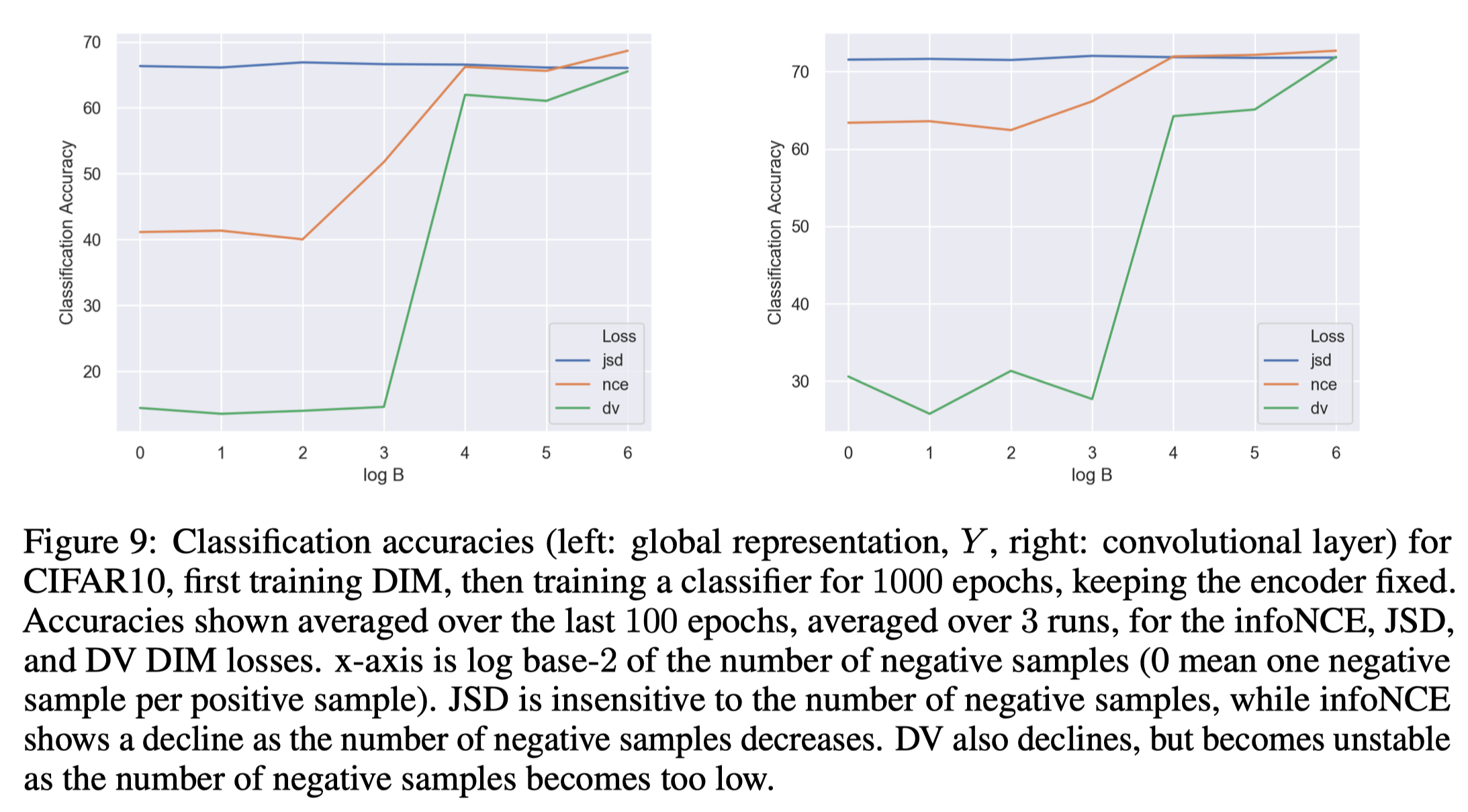
The InfoNCE objective experimentally performs best on downstream tasks among the three with large negative samples, but the performance drops quickly as we reduce the number of samples used for the estimation.
The JSD-based objective is insensitive to the number of negative samples and performs well in practice.
Deficiency of Traditional Pixel-level Representation Learning
Pixel-level representation-learning algorithms could be detrimental when only a small fraction of the bits of the signal actually matter at a semantic level. Such issues become more apparent when it comes to the representation learned by generative models: as the dimension of the data becomes large, the objectives of generative models become dominated by the pressure to represent all of the pixels well, whereas it may not leave sufficient dimensions to capture the important characteristics of the distribution. In particular, generative models must represent all statistical variability in the data in order to generate (or even discriminate) properly, and much of this variability could be unimportant and even detrimental to the suitability of the representation for downstream tasks.
R Devon Hjelm et al. [1] argue that representation learning should be more directly in terms of their information content and statistical or structural constraints. To address the first quality, the authors propose learning unsupervised representations by maximizing mutual information. To address the second, they consider adversarially matching a prior to imposing structural constraints on the learned representation.
DIM
DIM defines an encoder network that distills a high-level representation and multiple discriminators for different objectives. In this section, we will walk through all these networks, along with their corresponding objectives.
Encoder Network
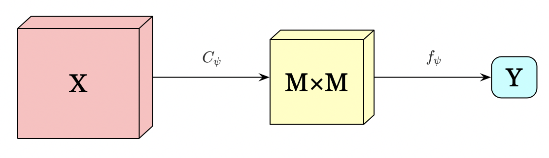
The encoder network, \( E_\psi=f_{\psi}\circ C_{\psi} \), first encodes the input \(X\) into an \(M\times M\) feature map, then summarizes this feature map into a high-level feature vector, \(Y=E_{\psi}(X)\).
Global Mutual Information Maximization
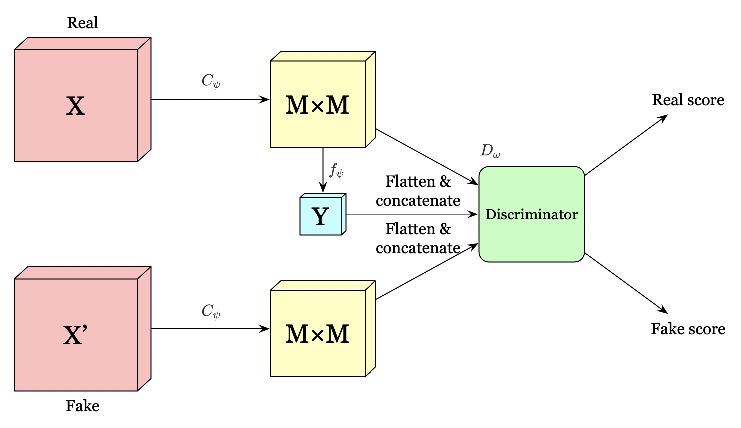
The above figure illustrates a global structure for representation learning with mutual information maximization.
The global structure first flattens the \(M\times M\) feature map and concatenate it with \(Y\). We then pass this to the discriminator to maximizes the mutual information between the \(M\times M\) feature map and \(Y\) using the following objective
\[\begin{align} \max_{\psi, \omega} I_{\psi, \omega}(X, Y) \end{align}\]where \(I\) could be any objective function discussed in the previous section.
Notice that we could generate negative samples by combining \(Y\) with different images in the same batch to save additional computational overhead.
Local Mutual Information Maximization
The global mutual information maximization may introduce some dependence irrelevant to the task. For example, trivial noise local to pixels is useless for image classification, so a representation may not be benefit from this information if the end-goal is to classify. Moreover, since the capacity of the high-level representation is fixed, such irrelevant information may squeeze out some valuable information.
To eliminate the unwanted local noise, the authors suggest maximizing the average mutual information between the high-level representation \( Y \) and all local patches of the feature map (feature vectors in the \( M\times M \) feature map). Because now the high-level representation \(Y\) is encouraged to have high mutual information with all patches, this favors encoding aspects of the data that shares across patches. Experiments also verify the intuition that this encourages the encoder to prefer information shared across the input and significantly boosts classification performance.
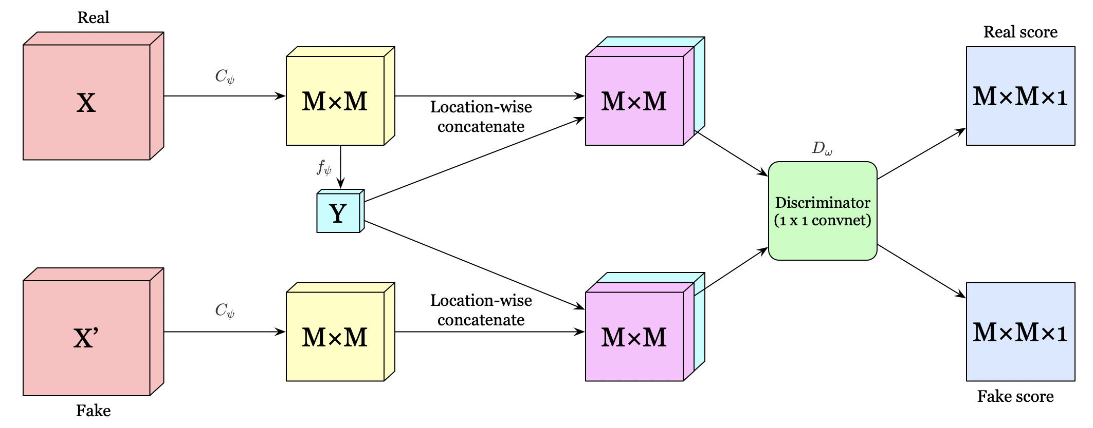
The authors propose two different architectures for the local objective. The first, depicted in the above figure, concatenate \(Y\) with the feature map at every location. A \(1\times 1\) convolutional discriminator is then used to score every feature vector in the location-wise concatenated \(M\times M\) feature map.
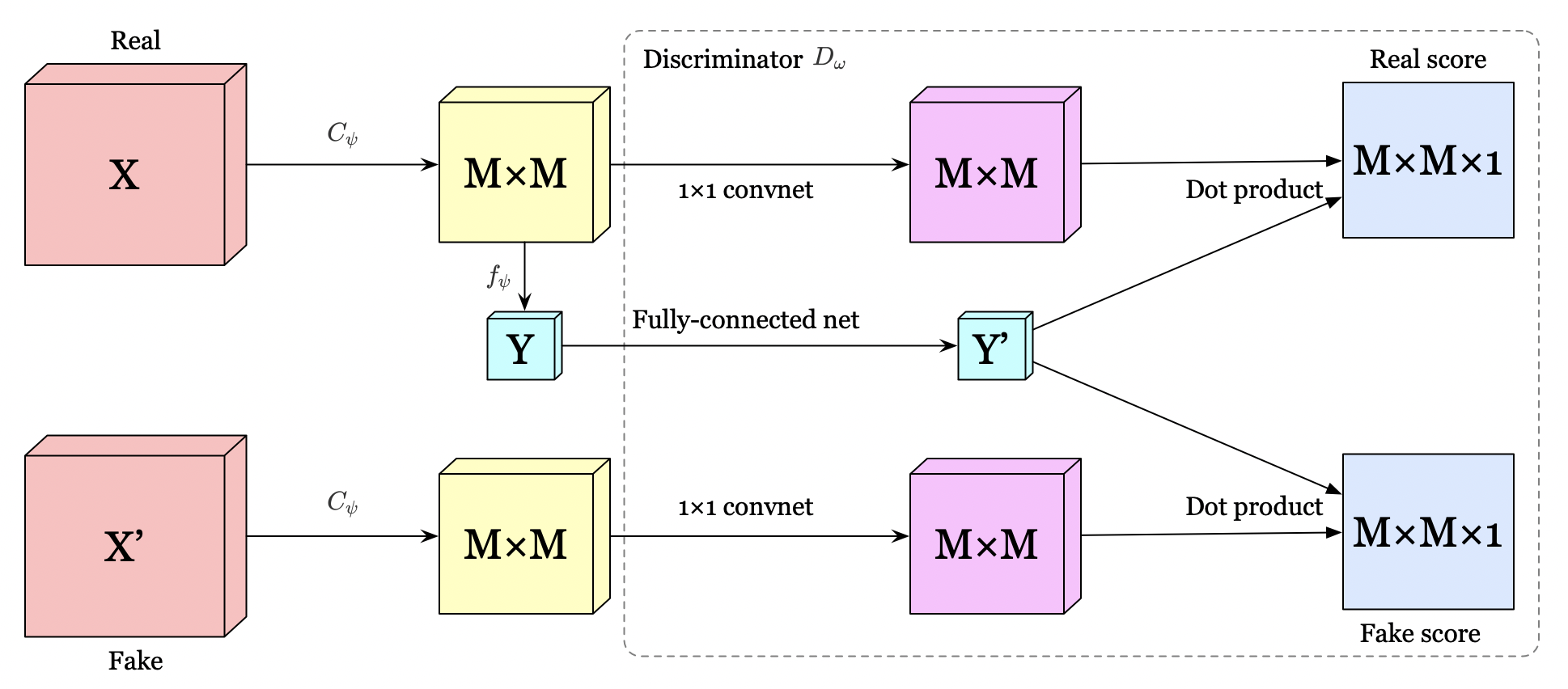
The other architecture, shown in Figure 4, further encodes the \(M\times M\) feature map and \(Y\) through a \(1\times 1\) convolutional network and a fully-connected network, respectively. We then take the dot product between the feature at each location of the feature map encoding and the encoded global vector for scores.
The objective used for local mutual information maximization is defined as
\[\begin{align} &\max_{\psi, \omega}{1\over M^2}\sum_{i=1}^{M^2}I_{\psi, \omega}^{(i)}(X, Y) \end{align}\]where \(I^{(i)}\) could be any objective function discussed in the first section.
To reduce computational overhead, the fake samples are generated by shuffling the feature map at each location across a batch independently.
Python code for local mutual information maximization is appended at the end.
Potential Improvements from Myself :-)
In my humble opinion, local mutual information may still struggle for certain tasks if the main features \( Y \) tries to capture may not share across all local patches of the image. In this sense, it might be helpful, for some specific tasks such as classification, to extract regions of interest (e.g., via an RPN) in advance and then apply global mutual information maximization to those regions.
Match Representation to a Prior Distribution
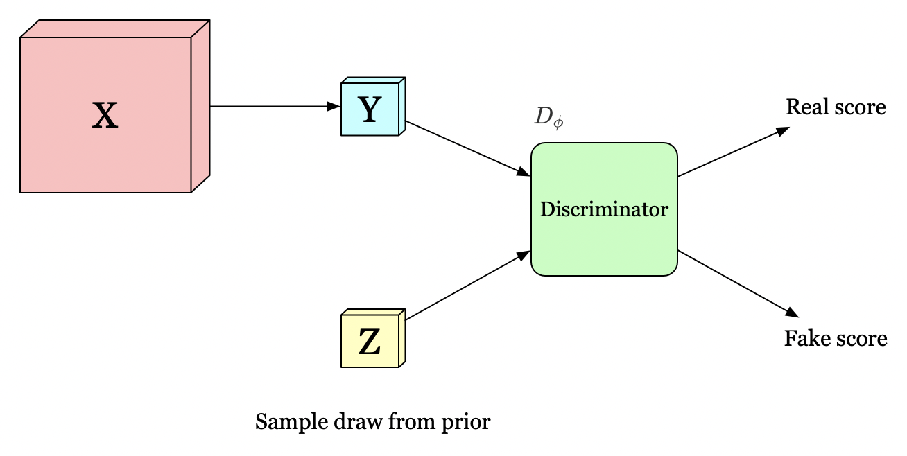
In order to satisfy the structural constraints, dim also matches the representation to a prior distribution \(P(Z)\). We define a new discriminator which distinguishes if the input distribution is from the output of the encoder or the prior distribution. The objective is simply a cross-entropy loss
\[\begin{align} \min_{\psi}\max_{\phi}D_\phi(Z\Vert Y)=E_{z\sim V}\left[ \log D_\phi(z)\right]+E_{x\sim p(x)}\left[\log (1-D_{\phi}(E_\psi(x)))\right] \end{align}\]The reason why we impose the structural constraints on \(Y\) is that, during the course of approximating to the prior \(Z\), we expect \(E_{\psi}\) to learn a representation with some desirable properties such as independence and disentanglement if the prior \(Z\) inherently owns such properties.
Put All Together
The objective for the whole DIM is
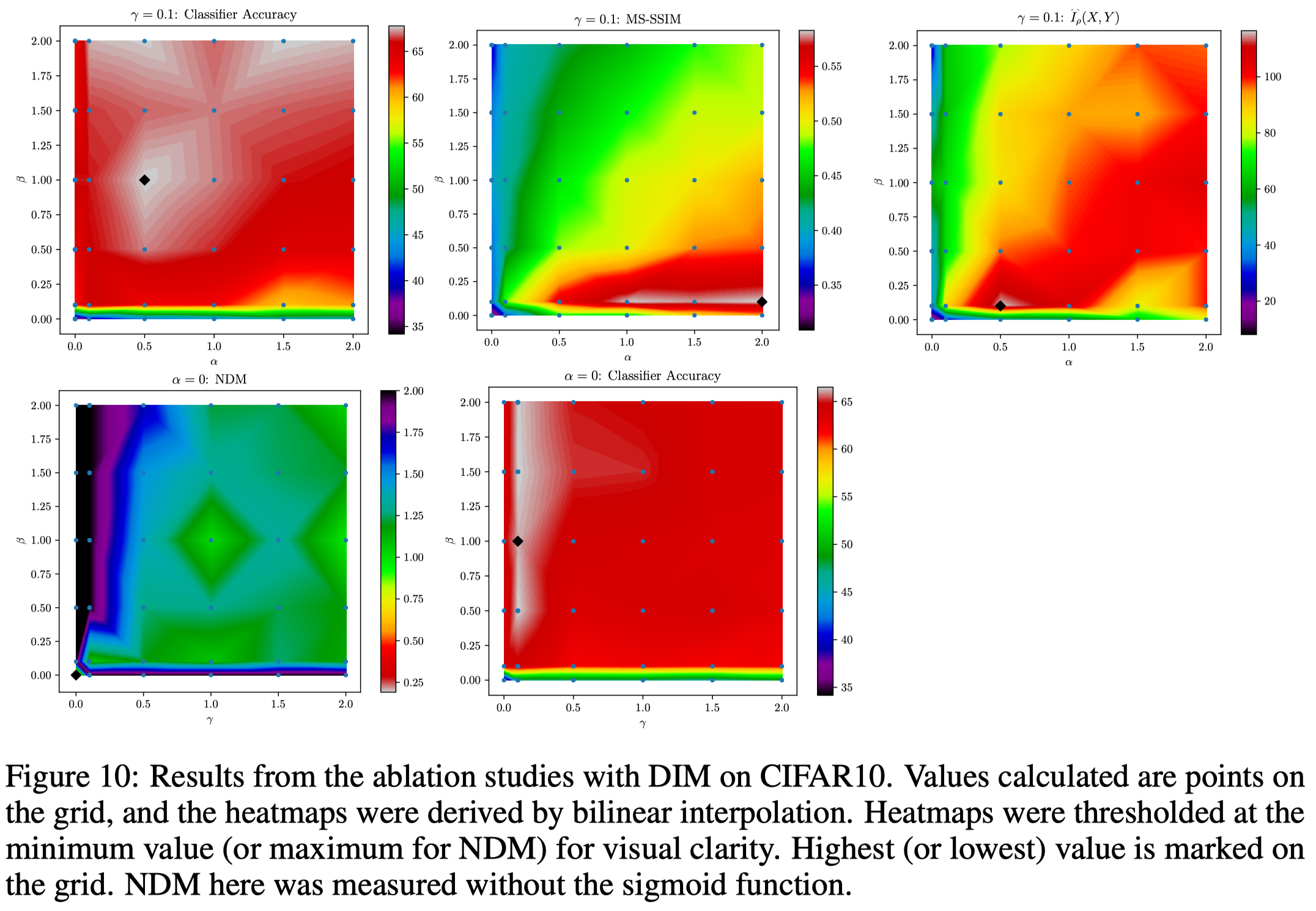
\[\begin{align} \max_{\psi, \omega_1, \omega_2}\left(\alpha I_{\psi, \omega_1}(X, E_{\psi}(X))+{\beta\over M^2}\sum_{i=1}^{M^2}I_{\psi, \omega_2}^{(i)}(X, E_{\psi}(X))\right) +\min_{\psi}\max_{\phi}\gamma D_\phi(V\Vert U_{\psi, P}) \end{align}\]where \( \alpha \), \( \beta \) and \( \gamma \) are hyperparameters. The following figure shows some ablation studies done by the authors, where \(y\)-axis is \(\beta\). In particular, we can see good classification performance is highly dependent on the local term, \(\beta\), while good reconstruction highly depends on the global term \(\alpha\). However, a small amount of \(\alpha\) helps in classification accuracy and a small amount of \(\beta\) improves reconstruction.
Implementation Details
Devon Hjelm et al. found using a nonlinearity (such as a sigmoid for a uniform prior) on the output representation, \(Y\), was important for performance on higher-dimensional datasets. ReLU activations from the feature map needed to be included in the mutual information estimation step for the approach to work well.
Supplementary Materials
Proof for the validity of JSD objective
In this sub-section we prove
\[\begin{align} D_{JS}(P(X,Y)\Vert P(X), Y)\ge2\log 2+E_{p(x,y)}\left[-\mathrm{sp}(-T(x, y))\right]-E_{p(x')p(y)}\left[\mathrm{sp}(T(x', y))\right]\tag {2} \end{align}\]First, we define the \( f \) divergence
\[\begin{align} D_f(P\Vert Q)=\int_x q(x)f\left({p(x)\over q(x)}\right)dx \end{align}\]then we replace the \( f \) function with the convex conjugate
\[\begin{align} D_{f}(P\Vert Q)&=\int_x q(x)\sup_{t\in \mathrm{dom}(f^\*)} \left\{ {p(x)\over q(x)}\cdot t- f^\*(t)\right\}dx\\\ &\ge\sup_{T(x)\in\mathrm{dom}(f^\*)}\left\{\int_xq(x) \left({p(x)\over q(x)}\cdot T(x)-f^\*(T(x))\right)dx\right\}\\\ &=\sup_{T(x)\in\mathrm{dom}(f^\*)}\left\{E_{x\sim p}\left[T(x)\right]-E_{x\sim q}\left[f^\*(T(x))\right]\right\} \tag{3} \end{align}\]the second step yields a lower bound for two reasons: 1. because of Jensen’s inequality when swapping the integration and supremum operations. 2. the class of functions \( T(x) \) may contain only a subset of all possible \( t \).
Since we aim to derive the Jensen-Shannon divergence, so we replace \( f(x) \) with \( -(x+1)\log{1+x\over 2}+x\log x \) (Sebastian Nowozin et al. [3]). Now we infer \( f^*(t) \)
\[\begin{align} f^\*(t)&=\sup_{x\in \mathrm{dom}(f)} \left\{t\cdot x- f(x)\right\}\\\ &=\sup_{x\in \mathrm{dom}(f)}\left\{t\cdot x+(x+1)\log{1+x\over 2}-x\log x \right\}\\\ &=\sup_{x\in \mathrm{dom}(f)}\left\{\phi_t(x) \right\}\quad where\ \phi_t(x)=t\cdot x+(x+1)\log{1+x\over 2}-x\log x\tag {4} \end{align}\]This suggests that \( f^*(t) \) is obtained when \( \phi_t(x) \) is at the maximum, so we set the derivative of \( \phi_t(x) \) to zero and have
\[\begin{align} \phi_t'(x)&=0\\\ t+\log{x+1\over 2}+1-\log x-1&=0\\\ x&={e^t\over 2-e^t}\tag {5} \end{align}\]Sticking Eq.\( (5) \) back to Eq.\( (4) \), we get the convex conjugate of \( f \)
\[\begin{align} f^\*(t)&=t\cdot { {e^t\over 2-e^t}}-\left({2\over 2-e^t}\right)\log\left(2-e^t\right)-{e^t\over 2-e^t}\log \left(e^t\over 2-e^t\right)\\\ &=-\log(2-e^t)\tag {6} \end{align}\]Then we define \(T(x)=\log2-\log\left(1+e^{-T’(x)}\right) \) and substitute it back to Equation \((3)\). This gives us
\[\begin{align} D_{JS}(P\Vert Q)&\ge\sup\left\{ E_{x\sim P}\left[\log 2-\log\left(1+e^{-T'(x)}\right)\right]-E_{x\sim Q}\left[ -\log\left(2-e^{\log2-\log(1+e^{-T'(x)})}\right) \right] \right\}\\\ &=\sup\left\{ E_{x\sim P}\left[\log 2-\log\left(1+e^{-T'(x)}\right)\right]-E_{x\sim Q}\left[ -\log\left(2-{2\over1+e^{-T'(x)}}\right) \right] \right\}\\\ &=\sup\left\{\log 2+ E_{x\sim P}\left[-\log\left(1+e^{-T'(x)}\right)\right]-E_{x\sim Q}\left[ \log\left({1+e^{T'(x)}}\right) \right]+\log2 \right\}\\\ &=\sup\left\{\log 2 + E_{x\sim P}\left[-\mathrm{sp}\left({-T'(x)}\right)\right]+\log 2-E_{x\sim Q}\left[ \mathrm{sp}\left({ {T'(x)}}\right) \right] \right\}\tag {7} \end{align}\]The only thing left to do is just to replace relative symbols with those in Eq.\( (2) \) and the proof completes.
In practice, we generally further divide the last term for numerical stability:
\[\begin{align} \mathrm{sp}(T'(x))&=\log\left(1+e^{T'(x)}\right)\\\ &=\log\left(1+e^{-T'(x)}\right) + T'(x) \end{align}\]Aware of that \( -\mathrm{sp}(x) = \log\sigma(-x) \), we could further express \( (7) \) as follows
\[\begin{align} D_f(P\Vert Q)\ge\sup\left\{\log 2 + E_{x\sim P}\left[\log\sigma\left(T'(x)\right)\right]+\log 2+E_{x\sim Q}\left[\log\sigma\left(-T'(x)\right) \right]\right\} \end{align}\]Proof InfoNCE is a lower bound on Mutual Information
we first rewrite InfoNCE
\[\begin{align} I^{\mathrm{InfoNCE}}(X; Y)&= E_{p(x, y)}\left[T(x,y)-\log\sum_{x'\sim p(x)}e^{T(x',y)}\right]\\\ &=E_{p(x,y)}\left[\log{e^{T(x,y)}\over\sum_{x'}e^{T(x',y)}}\right]\\\ &=E_{p(x,y)}\left[\log{f(x,y)\over\sum_{x'}f(x',y)}\right] \end{align}\]Optimizing this objective, the fraction approximates the probability of \(E_\psi(x)=y\) for a specific \(y\) and some \(x\) drawn from \(p(x)\). We denote this optimal probability as \(p(E_\psi(x)=y\vert X,y)\), and apply Bayes’ theorem
\[\begin{align} p(E_\psi(x)=y|X,y)&={p(E_\psi(x)=y, X|y)\over\sum_{i=1}^Np(E_\psi(x_i)=y,X|y)}\\\ &={p(x|y)\prod_{x_l\ne x}p(x_l)\over \sum_{i=1}^Np(x_i|y)\prod_{x_l\ne x_i}p(x_l)}\\\ &={ {p(x|y)\over p(x)}\over\sum_{i=1}^N{p(x_i|y)\over p(x_i)}} \end{align}\]Thus, the optimal value of \(f(x,y)\) is given by \(p(x\vert y)\over p(x)\).
Python Code for Local Mutual Information Maximization
def dim(feature_map, z, batch_size=None, log_tensorboard=False):
    with tf.variable_scope('loss'):
        with tf.variable_scope('local_MI'):
            E_joint, E_prod = _score(feature_map, z, batch_size)

            local_MI = E_joint - E_prod

    return local_MI

def _score(feature_map, z, batch_size=None):
    with tf.variable_scope('discriminator'):
        T_joint = _get_score(feature_map, z, batch_size)
        T_prod = _get_score(feature_map, z, batch_size, shuffle=True)

        log2 = np.log(2.)
        E_joint = tf.reduce_mean(log2 - tf.math.softplus(-T_joint))
        E_prod = tf.reduce_mean(tf.math.softplus(-T_prod) + T_prod - log2)

    return E_joint, E_prod

def _get_score(feature_map, z, batch_size=None, shuffle=False):
    with tf.variable_scope('score'):
        height, width, channels = feature_map.shape.as_list()[1:]
        z_channels = z.shape.as_list()[-1]

        if shuffle:
            feature_map = tf.reshape(feature_map, (-1, height * width, channels))
            if batch_size is None:
                feature_map = tf.random.shuffle(feature_map)
            else:
                feature_map = _local_shuffle(feature_map, batch_size)
            feature_map = tf.reshape(feature_map, (-1, height, width, channels))
            feature_map = tf.stop_gradient(feature_map)

        # expand z
        z_padding = tf.tile(z, [1, height * width])
        z_padding = tf.reshape(z_padding, [-1, height, width, z_channels])

        feature_map = tf.concat([feature_map, z_padding], axis=-1)

        scores = _local_discriminator(feature_map, shuffle)
        scores = tf.reshape(scores, [-1, height * width])

    return scores

def _local_discriminator(feature_map, reuse):
    with tf.variable_scope('discriminator_net', reuse=reuse):
        x = tf.layers.conv2d(feature_map, 512, 1)
        x = tf.nn.relu(x)
        x = tf.layers.conv2d(feature_map, 512, 1)
        x = tf.nn.relu(x)
        x = tf.layers.conv2d(feature_map, 1, 1)
        x = tf.nn.relu(x)

    return x

def _local_shuffle(x, batch_size):
    with tf.name_scope('local_shuffle'):
        _, d1, d2 = x.shape
        d0 = batch_size
        b = tf.random_uniform(tf.stack([d0, d1]))
        idx = tc.framework.argsort(b, 0)
        idx = tf.reshape(idx, [-1])
        adx = tf.range(d1)
        adx = tf.tile(adx, [d0])

        x = tf.reshape(tf.gather_nd(x, tf.stack([idx, adx], axis=1)), (d0, d1, d2))

    return x
References
[1] R Devon Hjelm et al. Learning deep representations by mutual information estimation and maximization
[2] Aaron van den Oord et al. Representation Learning with Contrastive Predictive Coding
[3] Sebastian Nowozin, et al. f-GAN: Training Generative Neural Samplers using Variational Divergence Minimization