
Tabble of Contents
- Mutual Information
- Mutual Information Neural Estimation
- Applications of MINE
- Supplementary Materials
Mutual Information
The general definition for the mutual information is
\[\begin{align} I(X;Z)=H(X) - H(X|Z)=H(Z)-H(Z|X)=I(Z;X) \end{align}\]where the Shannon entropy \( H(X) \) quantifies the uncertainty in \( X \) and the conditional entropy \( H(X\vert Z) \) the uncertainty in \( X \) given \( Z \).
There are three slightly different interpretations for the mutual information:
- Formally, mutual information captures the statistical dependence between random variables. (In contrast, the correlation coefficient only captures the linear dependence).
- Intuitively, the mutual information between \( X \) and \( Z \) describes the amount of information learned from knowledge of \( Z \) about \( X \) and vice versa.
- The direct interpretation is that it’s the decrease of the uncertainty in \( X \) given \( Z \) or the other way around.
Mutual information is also equivalent to the KL-divergence between the joint probability \( P(X, Z) \) and the product of the marginals \( P(X)\otimes P(Z) \):
\[\begin{align} I(X; Z)=D_{KL}(P(X,Z)\Vert P(X)\otimes P(Z))\tag{1}=I(Z;X) \end{align}\]The proof will be shown later here. The intuition behind this KL-divergence is that the more different the joint is from the product of the marginals, the stronger the dependence between \( X \) and \( Z \) is.
MINE Algorithm
MINE estimator gives the greatest lower-bound of the mutual information \( I(X; Z) \) by computing.
\[\begin{align} \sup_{T:\Omega\rightarrow\mathbb R}\mathbb E_{P(X,Z)}[T]-\log\mathbb E_{P(X)\otimes P(Z)}[e^T]\tag {2} \end{align}\]where \( T \) could be any function that takes as input \( x \) and \( z \) and outputs a real number. A detailed proof will be given later here. This greatest lower bound suggests that we are free to use any neural network to approximate the mutual information and, thanks to the expressive power of the neural network, such an approximation could gain arbitrary accuracy. The following algorithm does exactly what we just described, where \( \theta \) represents the net parameters
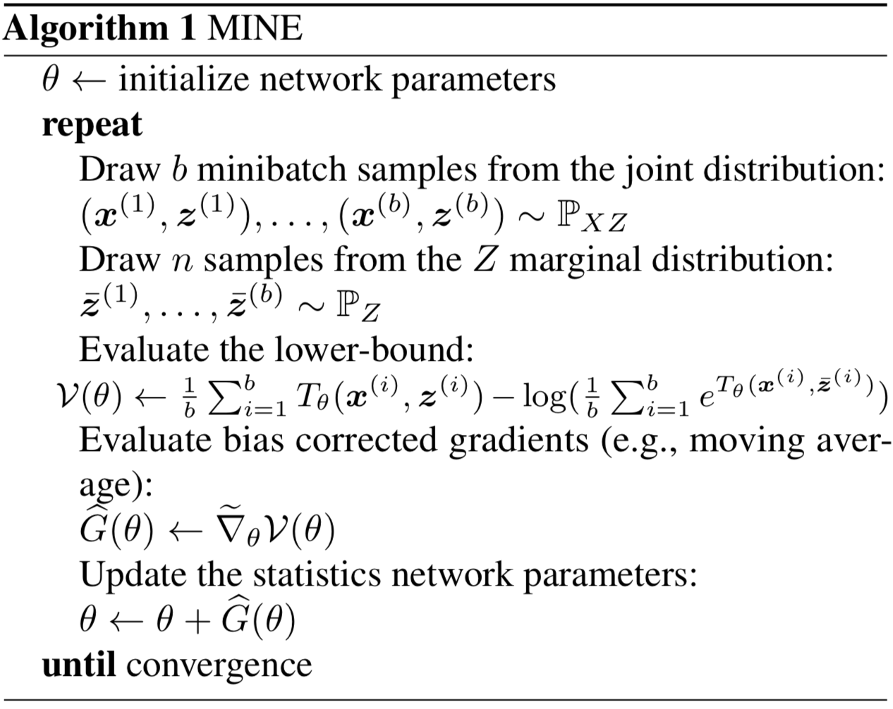
The gradient of \( \mathcal V(\theta) \) is
\[\begin{align} \nabla_\theta\mathcal V(\theta)=\mathbb E_{P(X, Z)}\left[\nabla_\theta T_\theta\right]-{\mathbb E_{P(X)\otimes P(Z)}\left[e^{T_\theta}\nabla_\theta T_\theta\right]\over \mathbb E_{P(X)\otimes P(Z)}\left[e^{T_\theta}\right]} \end{align}\]which is biased (because of the expectation in the denominator and minibatch gradient computation), the authors suggest replacing the expectation in the denominator with an exponential moving average. For small learning rates, this improved MINE gradient estimator can be made to have an arbitrarily small bias. Another paper also proposes substituting Jensen-Shannon Divergence for KL divergence to avoid \( \log \) and thereby escape such bias.
Equitability
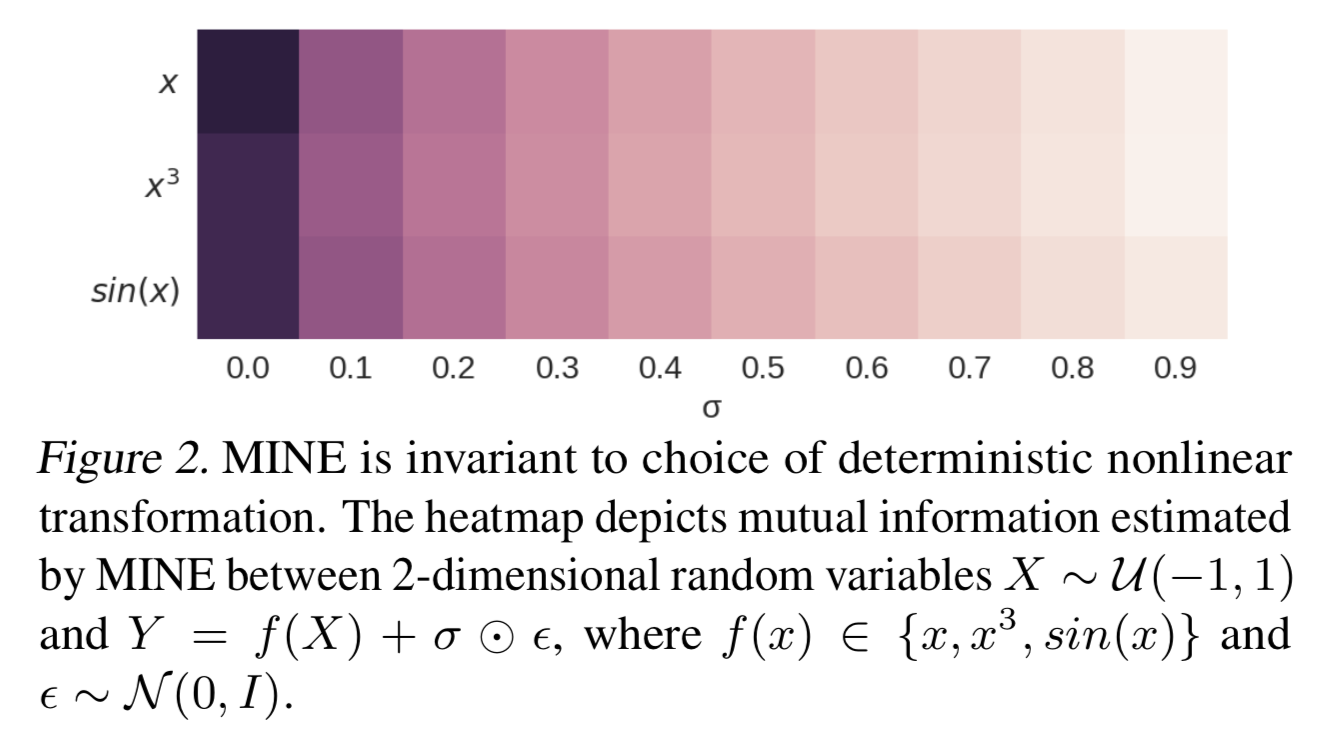
Let \( Y=f(X)+\sigma\odot\epsilon \), where \( f \) is a deterministic non-linear transformation and \( \epsilon \) is random noise. The property equitability of mutual information says that the mutual information between \(X\) and \(Y\), \(I(X; Y)\), is invariant to and should only depend on the amount of noise, \( \sigma \odot \epsilon \). That is, no matter \( f(x)=x \), \( f(x)=x^3 \) or something else, \( I(Y;X) \) stays approximately the same as long as \( \sigma \odot \epsilon \) remains unchanged. The following snapshot demonstrates MINE captures the equitability
Applications of MINE
Maximizing Mutual Information to Improve GANs
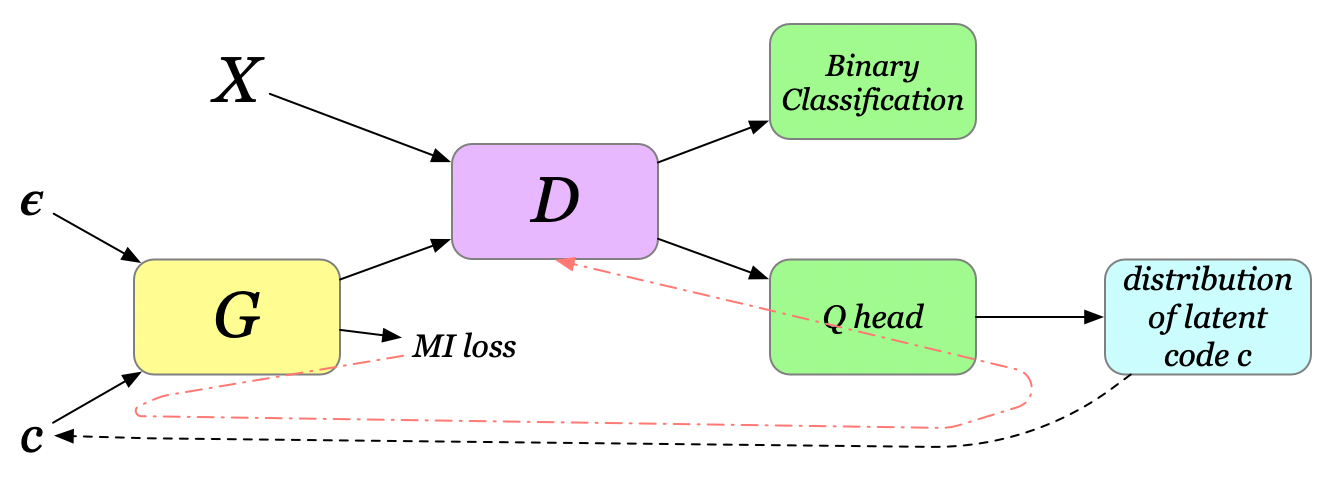
GANs commonly face mode collapse problem, where the generator fails to capture the diversity of training data. Let the latent vector of variables \( Z=[\epsilon, c] \), the concatenation of noise and code variables. The noise vector \( \epsilon \) is treated as a source of incompressible noise, while the latent code \( c \) captures the salient structured semantic features of the data distribution. In a vanilla GAN, the generator is free to ignore \( c \) since nothing enforces this dependency. To reinforce such dependency, we add an extra MI term to the generator loss as follows
\[\begin{align} L_G=L_\mu+L_m=-\mathbb E\left[ \log D(G([\epsilon, c])) \right] - \beta I(G([\epsilon, c]); c) \end{align}\]Notice that mutual information is unbounded so that \( L_m \) can overwhelm \( L_\mu \), leading to a failure mode of the algorithm where the generator puts all its attention on maximizing the mutual information and ignores the adversarial game with discriminator. The authors propose adaptively clipping the gradient from the mutual information so that its Frobenius norm is at most that of the gradient from the discriminator:
\[\begin{align} \min(\Vert g_\mu\Vert_F, \Vert g_m\Vert_F){g_m\over \Vert g_m\Vert_F} \end{align}\]BTW, \( c \) is not some magical variable coming out of nowhere; it’s sampled from an auxiliary distribution \( Q \), a network that gets optimized based on \( I(G([\epsilon, c]); c) \) through \(c\). In most experiments, \( Q \) shares all convolutional layers with discriminator \( D \), and have an additional final fully-connected layer to output parameters for conditional distribution \( Q(c\vert x) \), e.g., the mean and variance for a normal distribution. Furthermore, since \( c \) is sampled from the conditional distribution \( Q(c\vert x) \), we may also have to have recourse to the reparametrization trick in order to update \( Q \).
Maximizing Mutual Information to Improve BiGANs
A Brief Introduction to BiGANs
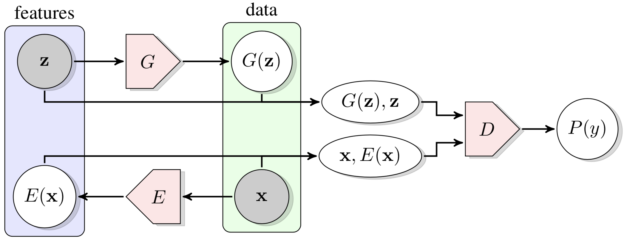
Bidirectional Generative Adversarial Networks, BiGANs, as the name suggests, is bidirectional in that the real data is encoded before being passed to the discriminator. The discriminator takes as input both the feature representations (\( \mathbf z \) and \( E(\mathbf x) \)) and the fully representative data (\( G(\mathbf z) \) and \( \mathbf x \)), distinguishing which from which. The generator and encoder collaborate to fool the discriminator by approaching \( E(\mathbf x) \) to \( \mathbf z \) and \( G(\mathbf z) \) to \( \mathbf x \).
BiGANs Cooperate with MINE
To reduce the reconstruction error, the authors prove that the reconstruction error, \( \mathcal R \), is bounded by
\[\begin{align} \mathcal R\le D_{KL}(q(\mathbf x, \mathbf z)\Vert p(\mathbf x, \mathbf z))-I_q(\mathbf x, \mathbf z)+H_q(\mathbf x)\tag {3} \end{align}\]where \( p \) concerns the generator and \( q \) the encoder. Detailed proof is appended at the end. From the above inequality, we can easily see that maximizing the mutual information between \( \mathbf x \) and \( E(\mathbf x) \) (albeit \( G(\mathbf z) \) and \( \mathbf z \) may seem more intuitive) minimizes the reconstruction error. Thus, we add the additional mutual information to the encoder loss and have
\[\begin{align} L_E=\mathbb E_{q(x, z)}\left[\log \left( 1-D(\mathbf x, E(\mathbf x))\right)\right]-\beta I_q(\mathbf x, \mathbf z) \end{align}\]Information Bottleneck
The gist of the information bottleneck is to summarize a random variable \( X \) so as to achieve the best tradeoff between accuracy and complexity. That is, we want to extract the most concise representation \( Z \) that captures the factors of \( X \) most relevant to the prediction \( Y \). The objective of the information bottleneck method is thus minimizing the Lagrangian
\[\begin{align} \min_{P(Z|X)}-I(Y;Z)+\beta I(X;Z)=\min_{P(Z|X)}H(Y|Z)+\beta I(X;Z)\\\ \end{align}\]where \( \beta \) is a Lagrange multiplier. The first term minimizes the uncertainty of \( Y \) given \( Z \), while the second term minimizes the dependency between \( X \) and \( Z \).
IMHO, the information bottleneck makes the representation \( Z \) more objective-oriented — i.e. it makes \( Z \) more specific to \( Y \), and meanwhile it provides \( Z \) addtional adaptability to the random variable \( X \). When it is applied to reinforcement learning, this may result in a policy less sensible to trivial changes of the environment and whereby improves transferability.
Supplementary Materials
Proof for \( (1) \)
\[\begin{align} I(X,Z)&=H(X)-H(X|Z)\\\ &=-\int_xp(x)\log p(x)dx+\int_{x,z}p(x,z)\log p(x|z)dxdz\\\ &=\int_{x,z}\bigl(-p(x,z)\log p(x) +p(x,z)\log p(x|z)\bigr)dxdz\\\ &=\int_{x,z}\left(p(x,z)\log {p(x,z)\over p(x)p(z)} \right)dxdz\\\ &=D_{KL}(P(X,Z)\Vert P(X)\otimes P(Z)) \end{align}\]Proof for \( (2) \) being the GLB of \( I(X; Z) \)
To show that \( (2) \) gives the GLB of \( I(X,Z) \), we just need to prove the following statement
\[\begin{align} \forall_{T:\Omega\rightarrow\mathbb R}\mathbb E_P[T]-\log(\mathbb E_Q[e^T])\le D_{KL}(P\Vert Q)\tag {4} \end{align}\]we first define the Gibbs distribution
\[\begin{align} G(x)&={1\over Z}e^{T(x)}Q(x)\\\ \mathrm {where}\ Z&=\mathbb E_Q\left[e^T\right] \end{align}\]then we represent the left side of \( (4) \) using the Gibbs distribution \( G \) we just defined
\[\begin{align} \mathbb E_P[T]-\log(\mathbb E_Q[e^T])&=\mathbb E_{x\sim P(x)}\left[T(x)-\log\mathbb E_Q[e^T] \right]\\\ &=\mathbb E_{x\sim P(x)}\left[\log {e^{T(x)}\over{\mathbb E_Q[e^T]}} \right]\\\ &=\mathbb E_{x\sim P(x)}\left[\log {e^{T(x)}Q(x)\over{\mathbb E_Q[e^T]}Q(x)} \right]\\\ &=\mathbb E_{x\sim P(x)}\left[\log {G(x)\over Q(x)}\right]\\\ &=\mathbb E_P\left[\log\left(G\over Q\right)\right] \end{align}\]now we compute the difference between the left and right side of \( (4) \)
\[\begin{align} \Delta=D_{KL}(P\Vert Q)-\left(\mathbb E_P[T]-\log(\mathbb E_Q[e^T])\right)&=\mathbb E_P\left[\log\left(P\over Q\right)\right]-\mathbb E_P\left[\log\left(G\over Q\right)\right]\\\ &=\mathbb E_P\left[\log\left( P\over G\right)\right]\\\ &=D_{KL}(P\Vert G) \end{align}\]The positivity of the KL-divergence ensures \( \Delta\ge 0 \). Therfore, Equation \( (4) \) always holds.
Proof for \( (3) \)
The reconstruction error is defined as
\[\begin{align} \mathcal R&=E_{x\sim q(x)}E_{z\sim q(z|x)}\left[-\log p(x|z)\right] \end{align}\]where \( p \) is the generator and \( q \) the encoder. This roughly measures the loss of fidelity that the generator recover \( x \) from \( z \) encoded by the encoder
\[\begin{align} \mathcal R&=E_{x\sim q(x)}E_{z\sim q(z|x)}\left[-\log p(x|z)\right]\\\ &=E_{x,z\sim q(x,z)}\left[\log {p(z)\over p(x, z)}\right]\\\ &=E_{x,z\sim q(x, z)}\left[\log {q(x,z)\over p(x,z)}-\log q(x,z)+\log p(z) \right]\\\ &=D_{KL}(q(x,z)\Vert p(x,z))+H_q(x,z)+ E_{z\sim q}\left[\log p(z)\right]\\\ &=D_{KL}(q(x,z)\Vert p(x,z))+H_q(x,z)-D_{KL}(q(z)\Vert p(z))-H_q(z)\\\ &=D_{KL}(q(x,z)\Vert p(x,z))-D_{KL}(q(z)\Vert p(z))+H_q(x|z)\\\ &=D_{KL}(q(x,z)\Vert p(x,z))-D_{KL}(q(z)\Vert p(z))-I_q(x,z)+H_q(x)\\\ &\le D_{KL}(q(x,z)\Vert p(x,z))-I_q(x,z)+H_q(x) \end{align}\]References
Mohamed Ishmael Belghazi et al. Mutual Information Neural Estimation
Xi Chen et al. InfoGAN: Interpretable Representation Learning by Information Maximizing Generative Adversarial Nets
Jeff Donahue et al. Adversarial Feature Learning
Ben Poole, Sherjil Ozair, Aaron van den Oord, Alexander A. Alemi, George Tucker. On Variational Bounds of Mutual Information