
Tabble of Contents
A Brief Introduction to Variational Autoencoder
In the variational autoencoder (VAE), we maximize the likelihood of the training data by maximizing the corresponding Evidence Lower BOund (ELBO) on the log data likelihood:
\[\begin{align} \max ELBO(x;\phi,\theta) &= \max E_{q_\phi(x)}\left[E_{z\sim q_\phi(z|x)}\left[ \log p_\theta(x|z)\right]-D_{KL}\left(q_\phi(z|x)\Vert p_\theta(z)\right)\right] \end{align}\tag{1}\]where the first term measures the reconstruction likelihood of generating \( x \) given \( z \) sampled from the approximate likelihood \( q_{\phi}(z\vert x) \), the output of the encoder network; the second term, acting as a regularizer, measures the difference between \( q_\phi (z\vert x) \) and \( p_\theta (z) \). It encourages the encoder output \( q_\phi(z\vert x^{(i)}) \) to be close to \( p_\theta(z) \). For a detailed derivation and explanation, please refer to my previous post.
\( \beta \)-VAE
The \( \beta \)-VAE is a variant of VAE, which attempts to learn a disentangled representation by further penalizing the KL term in the ELBO.
\[\begin{align} \max ELBO(x;\phi,\theta) &= \max E_{q_\phi(x)}\left[E_{z\sim q_\phi(z|x)}\left[ \log p_\theta(x|z)\right]-\beta D_{KL}\left(q_\phi(z|x)\Vert p_\theta(z)\right)\right]\tag {2} \end{align}\]where \( \beta>1 \). Since the latent representation sampled from \( p_\theta(z) \), which is generally defined as the standard norm distribution, is naturally independent and factorial. By enforcing \( q_\phi(z\vert x) \) to be close to \( p_\theta(z) \), we implicitly impose disentanglement on the latent representation sampled from \( q_\phi(z\vert x) \).
\( \beta \)-TCVAE
\( \beta \)-TCVAE (total correlation variational autoencoder) further explores the KL term in \( \beta \)-VAE, identifying the source of disentanglement:
\[\begin{align} &\min E_{q_\phi(x)}\left[D_{KL}\left(q_\phi(z|x)\Vert p_\theta(z)\right)\right]\\\ =&\min E_{q_\phi(x,z)}\left[\log{q_\phi(z|x)q_\phi(x)\over q_\phi(x)q_\phi(z)}+\log {q_\phi(z)\over \prod_jq_\phi(z_j)}+\log {\prod_jq_\phi(z_j)\over p_\theta(z)}\right]\\\ =&\min \left\{D_{KL}\left(q_\phi(x,z)\Vert q_\phi(x)q_\phi(z)\right)+D_{KL}\left(q_\phi(z)\Vert\prod_j q_\phi(z_j)\right)+\sum_jD_{KL}\left(q_\phi(z_j)\Vert p_\theta(z_j)\right)\right\} \end{align}\]The first term, \( D_{KL}\left(q_\phi(x,z)\Vert q_\phi(x)q_\phi(z)\right) \), is the mutual information between \( x \) and \( z \) (i.e., \( I(x;z) \)), describing the dependence between \( x \) and \( z \).
The second term, \( D_{KL}\left(q_\phi(z)\Vert\prod_j q_\phi(z_j)\right) \), referred to as the total correlation, is one of many generalization of mutual information to more than two random variables(i.e., \( I(z_1;z_2;\dots) \)). By minimizing this term we introduce statistical independence to latent variables.
The last term, \( \sum_jD_{KL}\left(q_\phi(z_j)\Vert p_\theta(z_j)\right) \), namely element-wise KL, is derived under the assumption that the latent vector sampled from the prior is internally independent, i.e., \( p_\theta(z)=\prod_j p_\theta(z_j) \). Penalizing this term forces individual latent variables to be close to their corresponding priors.
The biggest issue here is that we don’t know how to compute the marginal distribution \( q_\phi(z) \) — a naive Monte Carlo approximation based on a minibatch of samples from \( q(x) \)(or equivalently, \( p(x) \)) is very likely to underestimate \( q_\phi(z) \) since \( q_\phi(z\vert x) \) is generally very small except when \( x \) is where \( z \) came from. The authors propose using a weighted version for estimating the function \( \log q(z) \) during training, inspired by importance sampling. When provided with a minibatch of samples \( {x_1, x_2,\dots,x_M} \), we can use the estimator
\[\begin{align} E_{q_\phi(z)}\left[\log{q_\phi(z)}\right]\approx {1\over M}\sum_{i=1}^M\left[\log {1\over NM}\sum_{j=1}^Mq_\phi(z(x_i)|x_j)\right]\tag {3} \end{align}\]A detailed proof will be append at the end, so will the python code computing the total variation
Hierarchically Factorized VAE (HFVAE)
Similar to beta-VAE and beta-TCVAE, HFVAE also tries to encourage statistical independence between latent variables whereby learning disentangled representation.
The vanilla VAE and its variants discussed above use the log data likelihood, namely \( E_{z\sim q_\phi(z\vert x)}\left[\log{p_\theta(x)}\right] \), as their objectives. It does not have to be that way — We could also reinterpret the objective as minimizing the difference between the encoder joint probability \( q_\phi(z,x) \) and the decoder joint probability \( p_\theta(x,z) \), or equivalently, maximizing the negative of their KL divergence
\[\begin{align} &\max -D_{KL}\left({q_\phi(z, x)\Vert p_\theta(x,z)}\right)\\\ =&\max E_{q_\phi(x,z)}\left[\log{p_\theta(x,z)\over q_\phi(z, x)}\right]\\\ =&\max E_{q_\phi(x,z)}\left[\log{p_\theta(x,z)\over p_\theta(x)p_\theta(z)}+\log{q_\phi(z)q_\phi(x)\over q_\phi(z, x)}+\log{p_\theta(x)\over q_\phi(x)}+\log{p_\theta(z)\over q_\phi(z)}\right]\\\ =&\max E_{q_\phi(x,z)}\left[\log{p_\theta(x|z)\over p_\theta(x)}-\log{q_\phi(z|x)\over q_\phi(z)}\right]-D_{KL}(q_\phi(x)\Vert p_\theta(x))-D_{KL}(q_\phi(z)\Vert p_\theta(z))\tag {4} \end{align}\]This objective differs from \( (1) \) only by a constant term \( H(X) \), the Shannon entropy of \( X \) with the probability distribution \( q_\phi \):
\[\begin{align} &\max E_{q_\phi(x)}\left[E_{q_{\phi}(z|x)}\left[\log p_\theta(x|z)\right]-\beta D_{KL}\left(q_\phi(z|x)\Vert p_\theta(z)\right)\right]\\\ =&\max E_{q_\phi(z, x)}\left[\log{p_\theta(x,z)\over q_\phi(z|x)}\right],\quad \mathrm{let}\ \beta = 1\\\ =&\max E_{q_\phi(z, x)}\left[\log{p_\theta(x, z)\over q_\phi(z, x)}\right]+H_{q_\phi}(X) \end{align}\]Here we append a snapshot from the original paper for better illustration
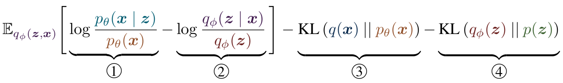
Next, we’ll explain each term in detail
- Term \( 1 \) intuitively maximizes the identifiability of the value \( z \) that generates \( x \). In other word, it enhances the connection between \( x \) and its corresponding \( z \) in the decoder network, and therefore we could anticipate that given \( z\sim q_\phi(z\vert x_i) \), then the reconstruction likelihood \( p_\theta(x_i\vert z) \) under the decoder network should be higher than the marginal likelihood \( p_\theta(x_i) \), which is averaged over \( z\sim p_\theta(z) \). Note that this term is intractable, since \( p_\theta(x) \) requires integral over \( z \).
- Term \( 2 \) minimizes the mutual information between \( x \) and \( z \) in the encoder network so as to regularize the first term for better generalization.
- Term \( 3 \) enforces consistency between the marginal distribution over \( x \), which draws the marginal reconstruction distribution \( p_\theta(x) \) close to the prior data distribution \( q_\phi(x) \).
- On the other hand, term \( 4 \) enforces consistency between the marginal distribution over \( z \), which draws the marginal encoding distribution \( q_\phi(z) \) close to the prior latent distribution \( p_\theta(z) \).
More to consider
- As we mentioned before, term \( 1 \) is intractable, however, if we combine it with term \( 3 \), they becomes the log reconstruction likelihood, which is tractable
-
In the encoder network, term \( 2 \) tries to minimize the mutual information between \( z \) and \( x \), while, in the decoder network, term \( 1 \) tries to maximize the identifiability of the values of \( z \) that generate \( x \). In other word, we tries to distill as little information \( z_i \) as possible from \( x_i \) in the encoder network, and meanwhile we also want this information \( z_i \) to be crucially representative of \( x_i \) so that the decoder network could possibly reconstruct \( x_i \) from it.
-
In practice, \( I(x, z) \) is often saturated to the upper bound \( H(X) \), no matter term \( 2 \) is included or not. This suggests that maximizing term \( 1 \) outweights the cost of term \( 2 \), at least for the encoder-decoder architecture.
-
We have testified that \( 4 \) differs from \( 2 \) only by a constant term (when \( \beta=1 \)), which means they should behave the same when \( \max \) is applied. Now let’s formally line them up:
This gives a similar intuition as \( \beta \)-TCVAE behind \( \beta \) penalty: increasing \( \beta \) penalizes the mutual information between \( x \) and \( z \), and draws the marginal encoding distribution \( q_\phi(x) \) close to the prior \( p_\theta(x) \), which should be well factorized for better disentanglement.
Take a deep look at term \( 4 \):
\[\begin{align} -D_{KL}(q_\phi(z)\Vert p_\theta(z))&=-E_{q_\phi(z)}\left[\log{q_\phi(z)\over\prod_dq_\phi(z_d)}+\log{\prod_d p_\theta(z_d)\over p_\theta(z)}+\log{\prod_dq_\phi(z_d)\over \prod_dp_\theta(z_d)}\right]\\\ &=E_{q_\phi(z)}\left[\log {p_\theta(z)\over \prod_dp_\theta(z)}-\log {q_\phi(z)\over \prod_d q_\phi(z_d)}\right]-\sum_dD_{KL}(q_\phi(z_d)\Vert p_\theta(z_d))\tag {5} \end{align}\]as we’ve seen before, the second term is the total correlation. The authors further propose recursively decomposing the last KL term to obtain more detailed factorization. Interested readers could refer to the paper for more details. I omit it here since I humbly think it is hard to decide a suitable size of the sub-variables \( z_d \), since we have no idea how much space is well suited for the factorization.
Supplementary Materials
Proof for \( (3) \)
Let \( B_M={x_1, \dots, x_M} \) be a minibatch of \( M \) indices where each element is sampled i.i.d. from \( p(x) \), so for any sampled batch instance \( B_M \), \( p(B_M)={1\over N}^M \). Let \( r(B_M\vert x) \) denote the probability of a sampled minibatch where one of the elements is fixed to be \( x \) and the rest are sampled i.i.d. from \( p(x) \). This gives \( r(B_M\vert x)={1\over N}^{M-1} \). Now we compute the expected marginal distribution \( q(z) \)
\[\begin{align} &E_{q(z)}\left[\log{q(z)}\right]\\\ =&E_{q(z, x)}\left[\log E_{x'\sim p(x)}\left[q(z|x')\right]\right]\\\ =&E_{q(z, x)}\left[\log E_{p(B_M)}\left[{1\over M}\sum_{m=1}^Mq(z|x_m)\right]\right]\\\ \ge&E_{q(z, x)}\left[\log E_{r(B_M|x)}\left[{p(B_m)\over r(B_M|x)}{1\over M}\sum_{m=1}^Mq(z|x_m)\right]\right]\\\ =&E_{q(z, x)}\left[\log E_{r(B_M|x)}\left[{1\over NM}\sum_{m=1}^Mq(z|x_m)\right]\right]\\\ \ge&E_{q(z, x),r(B_M|x)}\left[\log{1\over NM}\sum_{m=1}^Mq(z|x_m)\right] \end{align}\]Some explanations:
- In step second, we compute the average distribution of \( z \) given \( x \) from a minibatch and then we take the expectation on minibatches
- The first inequality is due to \( r \) having a support that is a subset of that of \( p \) — a given \( x \) may not appear in some minibatch
- The last step follows from Jensen’s inequality \( E_{p(x)}[\log q(z\vert x)]\le \log E_{p(x)}[q(z\vert x)] \)
During training, when provided with a minibatch of samples, we can use the estimator
\[\begin{align} E_{q(z)}[\log q(z)]\approx{1\over M}\sum_{i=1}^M\left[\log\sum_{j=1}^Mq(z(x_i)|x_j) - \log(NM)\right] \end{align}\]Python code computing the total variation
def tc_loss(sample_z, mu, logsigma, batch_size, dataset_size, image_size=1):
    """
    Arguments:
    	sample_z [batch_size, z_dim]: z sampled from distribution N(mu, exp(2*logsigma))
    	mu [batch_size, z_dim]: mean
    	logsigma [batch_size, z_dim] : log of the standard deviation
    	batch_size: the size of the minibatch
    	dataset_size: the size of the dataset
    	image_size: the size of the image, used when MSE is used as the reconstruction error
    """
    # log(q(zi|xj))
    logqzi_condxj_expanded = log_normal(tf.expand_dims(sample_z, axis=1),
                                      tf.expand_dims(mu, axis=0),
                                      tf.expand_dims(logsigma, axis=0))

    # log(NM)
    constant = np.log(dataset_size * batch_size)

    # sum_i(log(q(zi))) = sum_i(log(sum_j(q(zi|xj))) - constant)
    logqzi_marginal_product = tf.reduce_sum(logsumexp(logqzi_condxj_expanded,
                                                     axis=1, keepdims=False)
                                           - constant, axis=1)

    # log(q(z|xj))
    logqz_condxj = tf.reduce_sum(logqzi_condxj_expanded, axis=2)
    # log(q(z)) = log(sum_j(q(z|xj))) - constant
    logqz = logsumexp(logqz_condxj, axis=1, keepdims=False) - constant
    # divided by image_size**2 if MSE is used as reconstruction loss
    TC_loss = tf.reduce_mean(logqz - logqzi_marginal_product) / (image_size**2)

    return TC_loss

def log_normal(sample, mu, logsigma):
    """ Compute a Gaussian distribution density with mean mu and standard deviation exp(logsigma)

    Arguments:
        sample: x
        mu: mean
        logsigma: log of the standard deviation
    """
    log2pi = tf.constant([np.log(2 * np.pi)])           # log(2pi)
    inverse_sigma = tf.exp(-logsigma)                   # 1/sigma
    tmp = (sample - mu) * inverse_sigma                 # (x - mu)/sigma

    return -0.5 * (tmp**2 + 2 * logsigma + log2pi)      # log(N(x; mu, sigma**2))

def logsumexp(value, axis=None, keepdims=False):
    """ Compute the log of the sum of the exp of value

    Arguments:
    	value: tensor for which we compute logsumexp
    	axis: axis along which we apply sum
    	keepdims: if true, retains reduced dimensions with length 1.
    """
    if axis is not None:
        max_value = tf.reduce_max(value, axis=axis, keepdims=True)
        value = value - max_value    # for numerical stability
        if keepdims == False:
            max_value = tf.squeeze(max_value)
    else:
        max_value = tf.reduce_max(value)
        value = value - max_value

    return max_value + tf.log(tf.reduce_sum(tf.exp(value),
                                            axis=axis, keepdims=keepdims))
References
Irina Higgins et al. β-VAE: Learning Basic Visual Concepts with a Constrained Variational Framework
Tian Qi Chen et al. Isolating Sources of Disentanglement in Variational Autoencoders
Babak Esmaeili et al. Structured Disentangled Representations