
Tabble of Contents
- GANs for Data Generation
- GANs for Semi-supervised Learning
- Guidelines for Stable Deep Convolutional GANs
- Improved Techniques for Training GANs
Introduction
GAN is a popular generative model, introduced by Ian Goodfellow et al. in 2014. GAN is comprised of two competing networks, a generator \( G \) and a discriminator \( D \). These two networks contest against each other: the generator makes fake data trying to fool the discriminator; the discriminator receives both real and fake data and distinguish whether the data received is real or fake.
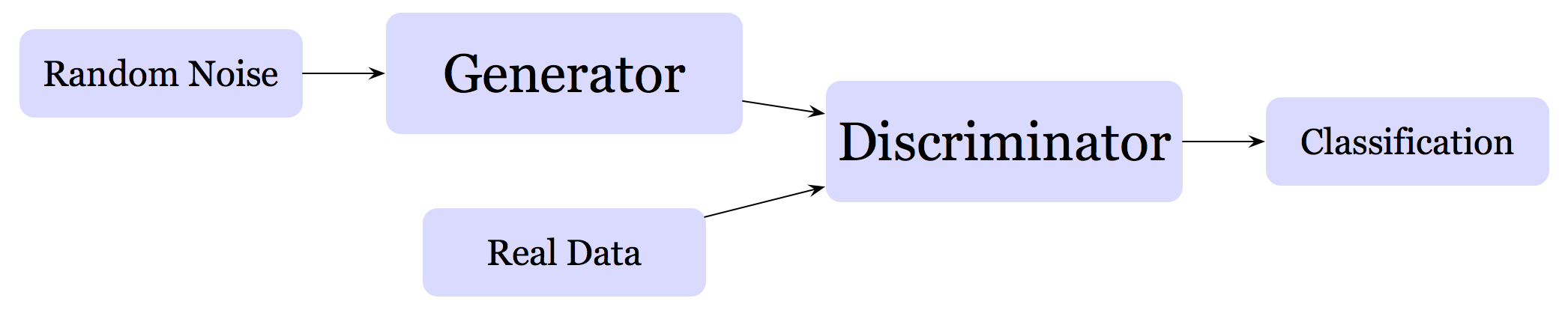
This architecture can mainly be used in two ways:
- For generating data: we throw away the discriminator at the end of the training and use the generator to generate data
- For semi-supervised learning: we throw away the generator after the training is done, and use the discriminator as a classifier. Some experiments show that a classifier trained in this way will generalize much better than a traditional classifier trained on only one source of data
GANs for Data Generation
GANs used for data generation are quite straightforward. The generator is mainly a network (upsampling net for images), which takes as input a random noise \( z \) and outputs data fed into discriminator. The discriminator takes as input both real and fake data and outputs a probability, which indicates whether the input is real or fake.
There are some things needed to be aware of:
- The distribution of \( z \) used in test time must be the same as that in training time, since the generator mainly tries to approximate \( P(x\vert z) \) to \( P(x) \), where \( P(x\vert z) \) is represented by the generation network and \( P(x) \) is the real data distribution
- The output of the generator should have the same value range as the real data have. For example, if we scale the real image data to range \( (-1, 1) \), then we should apply \( tanh \) to the output of the generator so that the output data are in range \( (-1, 1) \) too.
- We use label smoothing for the real image to help the discriminator generalize better. Specifically, we reduce the labels for the real data a bit from \( 1 \) to \( 0.9 \)
GANs for Semi-supervised Learning
Compared to GANs for data generation, GANs for semi-supervised learning is quite involved. The main reason is that we now have three data sets which are going to be fed into discriminator: The labeled real data, the unlabeled real data, and the fake data. Now let’s see what changes we have to make in order for the discriminator to harness semi-supervised learning.
Discriminator
-
We don’t apply batch normalization on some hidden layer (e.g., the second last layer). Feature maps output by this layer will later be used to compute the generator loss.
-
There are two choices for the output of the discriminator: one is to simply define one class for each real category, the other is to define an extra class for the fake category. These two are identical since \( \mathrm{softmax} \) remains the same if we subtract a general function \( f \) from each output logit — in this case, we set \( f=logit_{fake} \), and then we have \( logit_{fake} - logit_{fake}\equiv0 \).
-
We should derive the binary probability of data being real given input from the multiclass logits. That is, we should have
working out the math, we have
\[logit_{binary}=\log \left(\sum_{i\in real\ classes}e^{logit_{i}}\right)-logit_{fake}\]where \( logit_i \) is the logit for class \( i \), and \( logit_{fake} \) is the logit for the fake class or \( 0 \) if we don’t define an extra class for it. Generally, we usually rewrite the \( \log \) part as below for numerical stability
\[\begin{align} \log \left(\sum_{i\in real\ classes}e^{logit_{i}}\right)&=\log \left(\sum_{i\in real\ classes}e^{logit_{i}-logit_{max}}\right) + logit_{max}\\\ logit_{max}&=\max_{i\in real\ classes}(logit_i) \end{align}\]Here is an exemplary python code implemented in tensorflow for the 2 and 3 mentioned above
# using extra class or not doesn't affect other implementation
if extra_class:
    real_logits, fake_logits = tf.split(class_logits, [num_classes, extra_class], axis=1)
    fake_logits = tf.squeeze(fake_logits)
else:
    real_logits = class_logits
    fake_logits = 0.
# binary logits
max_logits = tf.reduce_max(class_logits, axis=1, keepdims=True)

real_logits = real_logits - max_logits

binary_logits = tf.log(tf.reduce_sum(tf.exp(real_logits), axis=1)) + tf.squeeze(max_logits) - fake_logits
Loss
Discriminator Loss
The discriminator loss consists of three parts: the loss for the real unlabeled data, for the fake data, for the real labeled data. The tensorflow code to compute these losses are shown as below
d_loss_real = tf.losses.sigmoid_cross_entropy(tf.ones_like(binary_logits_on_data), binary_logits_on_data, label_smoothing=0.1)
d_loss_fake = tf.losses.sigmoid_cross_entropy(tf.zeros_like(binary_logits_on_samples), binary_logits_on_samples)
d_loss_class = tf.losses.softmax_cross_entropy(tf.one_hot(y, num_classes), class_logits_on_labeled_data)

d_loss = d_loss_real + d_loss_fake + d_loss_class
Generator Loss
The generator loss used here is quite different. It’s the feature matching loss invented by Tim Salimans et al, [2] at OpenAI, which minimizes the difference between the expected features on the data and the expected features on the generated samples. The features mentioned here should be the activation maps output by some hidden layer in the discriminator (the layer on which we said not applying batch normalization earlier). The reason to do so is to do divergence minimization between two lower-dimensional distributions since two high dimensional distributions often have disjoint support, which results in training unstable. (Hyunjik Kim et al. [3])
expected_data_features = tf.reduce_mean(data_features, axis=0)
expected_sample_feature = tf.reduce_mean(sample_features, axis=0)
g_loss = tf.norm(expected_data_features - expected_sample_feature)**2
Guidelines for Stable Deep Convolutinal GANs
Following guidelines are excerpted from Radford et al. [1].
-
Use stride convolutions for upsampling and downsampling
-
Use batch normalization in generator and discriminator except for the generator output layer and the discriminator input layer
-
Use fully-connected layers only at the input of the generator, which takes a uniform noise distribution, and output of the discriminator
-
Use ReLU in the generator for all layers except for the output, which uses tanh
-
Use Leaky ReLU(the slope of the leak is set to \( 0.2 \)) in discriminator
Improved Techniques for Training GANs
In 2016, Salimans et al [2] developed several interesting techniques toward convergent GAN Training, including label smoothing and feature matching we talked earlier. Now we’ll talk about several other interesting techniques introduced by the paper.
Minibatch Discrimination
One of the main failure modes for GAN is for the generator to produce similar-looking data (i.e., what the authors said the generator collapsed to a single point). If this happens, the generator will fail to reproduce the diversity of the real data, and instead output something mysterious. To avoid the collapse of the generator, the authors introduced minibatch discrimination which appended a distance metrics as side information to a feature vector in the discriminator. The distance metrics shows how similar (or close) examples in a minibatch is to each other. In this way, if the generator tries to fool the discriminator, the generated data in a minibatch must have a similar distribution as real data in a minibatch embodies.
The algorithm is loosely summarized as follows:
-
Take the feature vectors of a fully-connected layer \( f(x_i)\in\mathbb R^A \) and multiplies it by a tensor \( T\in \mathbb R^{A\times B\times C} \), which results in a matrix \( M_i\in \mathbb R^{B\times C} \)
-
Compute the similarity(closeness) of two samples \( x_i \) and \( x_j \), the \( L_1 \)-distance between the rows of the resulting matrix across samples and apply a negative exponential (\( b \) denotes row \( b \)):
- The output \( o(x_i) \), which measures the similarity of \( x_i \) with all other samples in the minibatch, is simply the sum:
- Concatenate the output \( o(x_i) \) to the original feature vectors \( f(x_i) \), and feed the result into the next layer of the discriminator.
# step 1
x = tf.layers.dense(f, num_kernels * kernel_dim)
x = tf.reshape(x, (-1, num_kernels, kernel_dim))
# step 2
diffs = tf.expand_dims(x, 3) - tf.expand_dims(tf.transpose(x, [1, 2, 0]), 0)
l1_norm = tf.reduce_sum(tf.abs(diffs), 2)
c = tf.exp(-l1_norm)
# step 3
o = tf.reduce_sum(c, 2)
# step 4
tf.concat([f, o], 1)
For the reasoning behind diffs, please refer to my answer to my own question on stackoverflow:-)
Minibatch Discrimination vs. Feature Matching
Minibatch discrimination introduced above allows us to generate visually appealing samples very quickly. On the other hand, feature matching was found to work much better if the goal is to obtain a strong classifier for semi-supervised learning.
Historically Averaging
Historically averaging adds an extra term to the loss function: \( \Vert \theta-{1\over t}\sum_{i=1}^t\theta[i]\Vert^2 \), where \( \theta[i] \) is the value of the parameters at past time \( i \)
This method may stop models circle around the equilibrium point and act as a damping force to converge the model.
Virtual Batch Normalization
Batch normalization causes the output of an input sample to be highly dependent on other samples in the same minibatch. To avoid this problem, VBN chooses a reference batch of samples at the start of training and then uses the statistics computed from this reference batch to normalize each sample during training.
VBN is computationally expensive since it requires running forward propagation on two mini-batches of data (since the parameters get updated after every back propagation, we need to recompute the output for the reference batch at each layer to keep it updated), so we use it only on the generator network.
Reference
- Alec Radford, Luke Metz, Soumith Chintala. Unsupervised Representation Learning with Deep Convolutional Generative Adversarial Network
- Tim Salimans, Ian Goodfellow, Wojciech Zaremba, Vicki Cheung, Alec Radford, Xi Chen. Improved Techniques for Training GANs
- Hyunjik Kim, Hyunjik Kim. Disentangling by Factorising
and so on.