
Introduction
A vanilla autoencoder encodes an input to a smaller dimensional representation, which stores latent information about the input data distribution. But the encoded vector (latent variable) in a vanilla autoencoder can only be mapped to the corresponding input. It cannot be used to generate similar images with some variability.
A variational autoencoder, on the other hand, is designed for such variability. It has a similar architecture as a vanilla autoencoder, except that it provides variability in two ways:
- The latent variable \( z \) is sampled from a distribution specified by the encoder network (recall in a vanilla autoencoder, \( z \) is directly output by the encoder)
- The decoder network also outputs a distribution \( p_\theta(x^{(i)}\vert z) \) from which \( x \) is sampled (in a vanilla autoencoder, the decoder network deterministically outputs something similar to the input \( x^{(i)} \))
Workflow
The figure below is a general architecture for a variational autoencoder
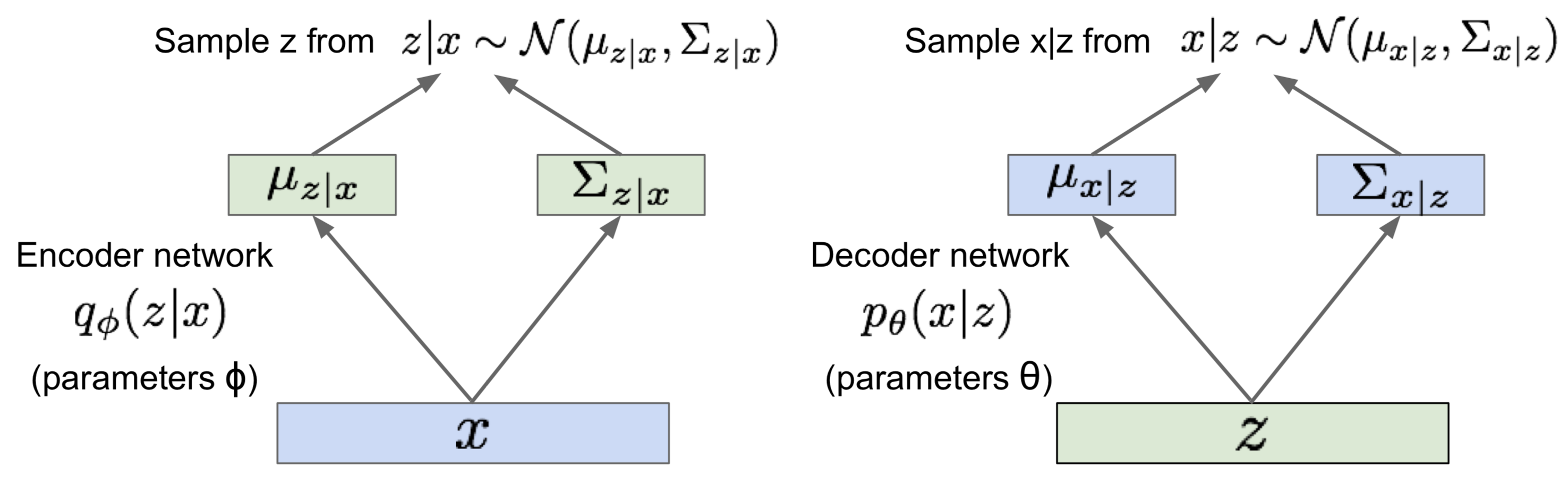
The encoder network (aka. recognition/inference network) takes \( x^{(i)} \) as input and outputs the mean and variance of a Gaussian distribution \( q_\phi(z\vert x) \) from which we sample the latent variable \( z \). The decoder network (aka. generation network), on the other hand, takes \( z \) as input and output the mean and variance of a Gaussian distribution for \( p_\theta(x^{(i)}\vert z) \).
Loss
In order to train a network, we want to maximize the likelihood of the training data. That is,
\[\begin{align} p_\theta(x^{(i)})=\int p_\theta(x^{(i)}|z)p_\theta(z)dz \end{align}\]where \( p_\theta(z) \) is simply the standard norm distribution \( \mathcal N(0,1) \). By maximizing \( p_\theta(x^{(i)}) \), we maximize the expected likelihood of generating \( x^{(i)} \) given latent variable \( z \) sampled from \( p_\theta(z) \), the standard normal distribution. This equation, however, is intractable since the integral suggests to compute \( p_\theta(x^{(i)}\vert z)p_\theta(z) \) for every \( z \).
Consider it in a Bayesian model, where we have
\[\begin{align} p_\theta(x^{(i)})={p_\theta(x^{(i)}|z)p_\theta(z)\over p_\theta(z|x^{(i)})} \end{align}\]In the above equation, although \( p_\theta(z\vert x^{(i)}) \) per se is also intractable, we can use an encoder network \( q_\phi(z\vert x^{(i)}) \) to approximate it. Some literature replaces \( p_\theta(x^{(i)}) \) with \( q_\phi(x^{(i)}) \) so as to be consistent with \( q_\phi(z\vert x^{(i)}) \). Since they both express the distribution of the data \( x^{(i)} \), just in different notations, we don’t bother to change the notation here.
Let’s take the expectation of the log of both sides
\[\begin{align} \log p_\theta(x^{(i)})&=E_{z\sim q_{\phi}(z|x^{(i)})}\left[\log {p_\theta(x^{(i)}|z)p_\theta(z)\over p_\theta(z|x^{(i)})}\right]\\\ &=E_z\left[\log {p_\theta(x^{(i)}|z)p_\theta(z)\over p_\theta(z|x^{(i)})}{q_\phi(z|x^{(i)})\over q_\phi(z|x^{(i)})}\right]\\\ &=E_z\left[\log {q_\phi(z|x^{(i)})\over p_\theta(z|x^{(i)})}-\log {q_\phi(z|x^{(i)})\over p_\theta(z)} + \log p_\theta(x^{(i)}|z) \right]\\\ &=D_{KL}\left(q_\phi(z|x^{(i)})\Vert p_\theta(z|x^{(i)})\right)-D_{KL}\left(q_\phi(z|x^{(i)})\Vert p_\theta(z)\right)+E_z\left[ \log p_\theta(x^{(i)}|z)\right] \end{align}\]Note that \( E_{z\sim q_\phi(z\vert x^{(i)})}\left[\log p_\theta(x^{(i)})\right]=\log p_\theta(x^{(i)}) \) since \( p_\theta(x^{(i)}) \) doesn’t depend on \( z \). We can see from the last step that the objective function consists of two KL divergences and a log likelihood. As we discussed before, the only thing intractable here is \( p_\theta(z\vert x^{(i)}) \) in the first KL divergence. Since KL divergence is guaranteed to be greater than or equal to \( 0 \), we could derive the Evidence Lower BOund(ELBO) on the log data likelihood
\[\begin{align} ELBO(x^{(i)};\phi,\theta) &= -D_{KL}\left(q_\phi(z|x^{(i)})\Vert p_\theta(z)\right)+E_z\left[ \log p_\theta(x^{(i)}|z)\right] \end{align}\]It’s called evidence lower bound since \( p_\theta(x^{(i)}) \) is generally called the evidence.
Because ELBO is the lower bound of \( \log p_\theta(x^{(i)}) \), the objective we want to maximize, it is quite intuitive to use the negative of the ELBO as a loss function.
\[\begin{align} \mathcal L(x^{(i)};\phi,\theta) &= -ELBO(x^{(i)};\phi,\theta)\\\ &= D_{KL}\left(q_\phi(z|x^{(i)})\Vert p_\theta(z)\right) - E_z\left[ \log p_\theta(x^{(i)}|z)\right] \end{align}\]The first term, the KL divergence, is a regularizer for \( \phi \), which encourages the approximate \( q_\phi(z\vert x^{(i)}) \) to be close to the prior \( p_\theta(z) \). This makes sense, because, as we said at the beginning, we want to maximize the likelihood of generating \( x^{(i)} \) given latent variable \( z \) sampled from \( p_\theta(z) \). In practice, if we represent \( q_\phi(z\vert x^{(i)}) \) and \( p_\theta (z) \) as Gaussians \( \mathcal N(\mu, \sigma^2) \) and \( \mathcal N(\mathbf 0, \mathbf I) \) respectively, this term can be integrated analytically:
\[\begin{align} D_{KL}\left(q_\phi(z|x^{(i)})\Vert p_\theta(z)\right) = -{1\over 2}\sum_{j=1}^J\left(1+2\log\sigma_j-\mu_j^2-\sigma_j^2\right) \end{align}\]where \( J \) is the dimensionality of \( z \).
The second term, the negative log data likelihood, is the reconstruction loss, which maximizes the likelihood that the generation network outputs \( x_i \) given \( z \) sampled from the approximate \( q_\phi(z\vert x^{(i)}) \). The probability is commonly defined as a multivariate Gaussian, i.e.
\[\begin{align} p_\theta(x^{(i)}|z) = \mathcal N(x^{(i)};\mu, \sigma^2) \end{align}\]where \( \mu \) and \( \sigma \) are computed by decoder network as the topmost figure illustrates
In general, this loss term cannot be backpropagated to the encoder parameter \( \phi \) since \( z \) is sampled from \( q_\phi(z\vert x^{(i)}) \). To solve this problem, we need to reparameterize the random variable \( z \) using a differentiable transformation \( g_\phi(\epsilon, x) \) and an auxiliary noise variable \( \epsilon \):
\[\begin{align} z=g_\phi(\epsilon, x), \epsilon \sim p(\epsilon) \end{align}\]In general, we choose \( \epsilon \) from the standard normal distribution, and we have
\[\begin{align} z=\mu+\sigma \cdot \epsilon, \epsilon \sim \mathcal N(\mathbf 0, \mathbf I) \end{align}\]