
Introduction
In this post, we will talk about region-based methods for object detection, and some auxiliary technique for region proposals. At last, I’ll briefly introduce the state-of-the-art instance segmentation architecture Mask R-CNN
Table of Contents
Preliminary
Graph-based Segmentation
Concept
For a graph \( G=(V,E) \), we define
-
the weight of an edge to be a non-negative measure of the dissimilarity between a pair of neighboring vertices
-
the internal difference of a component \( C \subseteq V \) to be the largest weight in the minimum spanning tree of the component, \( MST(C,E) \). That is
One intuition underlying this measure is that a given component \( C \) only remains connected when edges of weight at least \( \mathrm{Int}(C) \) are considered.
- the difference between two components \( C_1, C_2\subseteq V \) to be the minimum weight edge connecting the two components. That is,
- the minimum internal difference to be
where the threshold function \( \tau \) controls the degree to which the difference between two components must be greater than their internal difference in order for there to be evidence of a boundary between them. A threshould function introduced by the authors based on the size of the component is
\[\tau(C)=k/|C|\]This threshold function implies the requirement for strong evidence of a boundary for small component. In practice, \( k \) sets a scale of observation, in that a large \( k \) causes a preference for large components. Note, however, \( k \) is not a minimum component size. Smaller components are allowed when there is a sufficiently large difference between neighboring components
- the region comparison predicate to evaluate if there is evidence for a boundary between a pair of components
Algorithm
\[\begin{align} &\mathbf{Input}:\ \mathrm{Graph\ G=(V,E)}\\\ &\mathbf{Output}:\ \mathrm{Segmentation\ S}\\\ \\\ &\mathrm{Sort\ E\ in\ nondecreasing\ edge\ weight}\\\ &\mathrm{Initialize\ S=(C_1,C_2,...C_n),\ where\ each\ vertex\ v_i\ is\ in\ its\ own\ component}\\\ &\mathrm{For\ each\ edge\ e\ in\ E}\\\ &\quad \mathrm{(v_i,v_j)=e}\\\ &\quad \mathrm{If\ v_i\in C_i,\ v_j\in C_j, C_i\ne C_j\ and\ w(e)\le MInt(C_i, C_j)}\\\ &\quad \quad \mathrm{(i.e. The\ region\ comparison\ predicate\ is\ false)}\\\ &\quad \quad \mathrm{Merge\ C_i\ and\ C_j }\\\ &\mathrm{Return\ S} \end{align}\]Time complexity: \( n\log n \), where \( n \) is the number of edges
Selective Search
The graph-based segmentation cannot be used as region proposals for that
- Most actual objects contain \( 2 \) or more segmented parts
- Region proposals for occluded objects cannot be generated using this method
Selective search, built on the graph-based segmentation, is the algorithm designed to resolve these problems
Algorithm
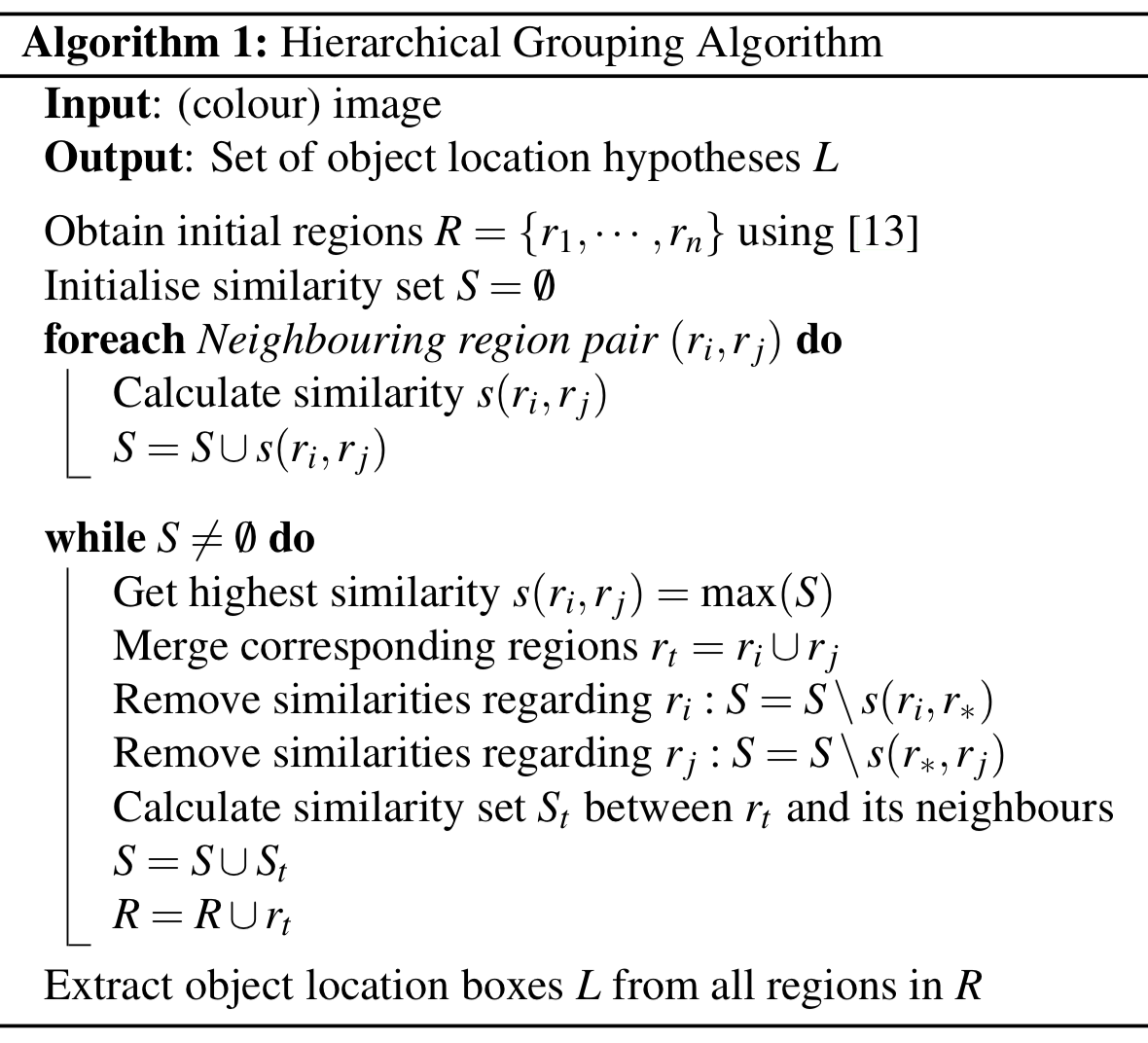
where [13] is the graph-based segmentation algorithm described before.
Similarity
Color Similarity
For each region, we obtain a color histogram for each channel using \( 25 \) bins. Then we concatenate histograms for all channels and normalize them using \( L_1 \) norm to form the color descriptor, \( C={c^1,\dots, c^n} \). Similarity is measured using the histogram intersection
\[\begin{align} s_{color}(r_i,r_j)=\sum_{k=1}^n\min(c^k_i,c^k_j) \end{align}\]The color descriptor can be efficiently propagated through the hierarchy by
\[\begin{align} C_t = {size(r_i)\times C_i+size(r_j)\times C_j\over size(r_i)+size(r_j)} \end{align}\]Texture Similarity
For each region, we take Gaussian derivatives in \( 8 \) directions for each channel. For each direction and for each channel, a \( 10 \)-bin histogram is computed resulting into a \( 10\times 8\times 3=240 \)-dimensional feature descriptor, \( T={t^1, \dots t^n} \) (assuming there are \( 3 \) channels). Then we normalize the descriptor using \( L_1 \) norm as we did before. Similarity and propagation through the hierarchy are computed just like the color descriptor:
\[\begin{align} s_{texture}(r_i,r_j)&=\sum_{k=1}^n\min(t_i^k,t_j^k)\\\ T_t &= {size(r_i)\times T_i+size(r_j)\times T_j\over size(r_i)+size(r_j)} \end{align}\]Size Similarity
Size similarity encourages small regions to merge early so as to prevent a single region from gobbling up all other regions, yielding all scales only at the location of this growing region and nowhere else. It’s defined as the fraction of the image that two regions jointly occupy
\[\begin{align} s_{size}(r_i,r_j)=1-{size(r_i)+size(r_j)\over size(image)} \end{align}\]where \( size(image) \) denotes the size of the image in pixels
Shape Compatibility
Shape compatibility measures how well region \( r_i \) and \( r_j \) fit into each other. That is, we try to merge regions in order to avoid any holes. Specifically, we define \( BB_{ij} \) to be the tight bounding box around \( r_i \) and \( r_j \). Shape compatibility is the fraction of the image contained in \( BB_{ij} \) which is not covered by the regions of \( r_i \) and \( r_j \)
\[\begin{align} s_{fill}(r_i,r_j)=1-{size(BB_{ij})-size(r_i)-size(r_j)\over size(image)} \end{align}\]Put All Together
The final similarity measure is a combination of the above four
\[\begin{align} s(r_i,r_j)=\ &a_1s_{color}(r_i,r_j)+a_2s_{texture}(r_i,r_j)+\\\ &a_3s_{size}(r_i,r_j)+a_4s_{fill}(r_i,r_j) \end{align}\]where \( a_i\in {0,1} \) denotes if the similarity measure is used or not
Region Proposal
We usually select the top \( N \) regions as region proposals, where \( N \) is around \( 1000-1200 \)
R-CNN
Workflow
i. Extract Region Proposals
In this step, it applies a region proposal method, such as selective search, to extract region proposals (around \( 2000 \)) and then wrap each region proposal so as to fit the fixed-size ConvNet input
ii. Extract Feature using ConvNet
To cope with the challenge that labeled data is too scarce to train a large ConvNet, the ConvNet used here are pre-trained on a large auxiliary dataset, and then followed by domain-specific fine-tuning on a small dataset. At the fine-tuning stage, the authors treat all region proposals with \( \ge 0.5 \) IoU overlap with a ground-truth box as positives for that box’s class and the rest as negatives
iii. Apply Linear SVMs to Classify Proposals
For training SVMs, the authors take only the ground-truth boxes as positive examples for their respective classes and label proposals with less than \( 0.3 \) IoU overlap with all instances of a class as a negative for that class. Proposals that fall into the grey zone (more than \( 0.3 \) IoU overlap, but are not ground truth) are ignored. This example-selection strategy is different from fine-tuning the ConvNet
Also note that there is an SVM for the background.
iv. Bounding-box Regression
For region proposals that have \( \ge 0.6 \) IoU overlap with a ground-truth box, we use their feature vectors, output from ConvNet, to train a regressor, which predicts an offset or a correction to the box of a region proposal. It is said that predicting offsets instead of coordinates simplifies the problem and makes it easier for the network to learn.
Mathematically, given a region proposal \( P=(P_x, P_y, P_w, P_h) \), where the first two specify the pixel coordinate of the center of proposal \( P \)’s bounding box and the second two specify log-space translation of the width and height of \( P \)’s bounding box, and the corresponding ground-truth bounding box \( G=(G_x, G_y, G_w, G_h) \), we define
\[\begin{align} \hat G_x&=P_wd_x(P)+P_x\\\ \hat G_y&=P_hd_y(P)+P_y\\\ \hat G_w&=P_w\exp(d_w(P))\\\ \hat G_h&=P_h\exp(d_h(P)) \end{align}\tag {1}\]Where \( d_x(P), d_y(P),d_w(P),d_h(P) \) are the correction predicted by the regressor.
Thereby, given \( \phi(P) \), the feature vectors for \( P \), the loss for the regressor is
\[\begin{align} L&=\sum_i^N\sum_k(t_k^i-\mathbf w_k^T\phi(P^i))^2+\lambda\left|\mathbf w\right|^2\\\ \end{align}\]where
\[\begin{align} \mathrm\ k\in\{x, y, w, h\}\\\ \begin{align} t_x&=(G_x-P_x)/P_w,&\quad t_w&=\log(G_w/P_w)\\\ t_y&=(G_y-P_y)/P_h, &\quad t_h&=\log(G_h/P_h)\\\ \end{align} \end{align}\]v. Object Detection at Test Time
At test time, SVMs score all feature vectors output by ConvNet. Then we apply a greedy non-maximum suppression (for each class independently) that rejects a region if it has a highly IoU overlap with a higher scoring selected region. At last, we rescale the remaining proposals according to \( (1) \)
Drawbacks
- Training is a multi-stage pipeline. The ConvNet, SVMs, and bounding-box regressors are trained separately.
- Training is expensive in time and space. Because of multi-stage training, the input features for SVM and bounding-box training have to be stored in the disk.
- Object detection is slow, since, at test time, ConvNet is applied to each region proposal, which leads to huge time complexity.
Fast R-CNN
Fast R-CNN tries to solve the drawbacks of R-CNN, it mainly differs from R-CNN in following aspects
- Fast R-CNN is an end-to-end network (achieved by replacing SVMs with a softmax classifier and applying ConvNet to an entire image). That means, training a fast R-CNN is single-stage, using a multi-task loss. This significantly reduces the time and space complexity of training
- It applies ConvNet to an entire image instead of each region proposal, which dramatically speeds up object detection at test time
Workflow
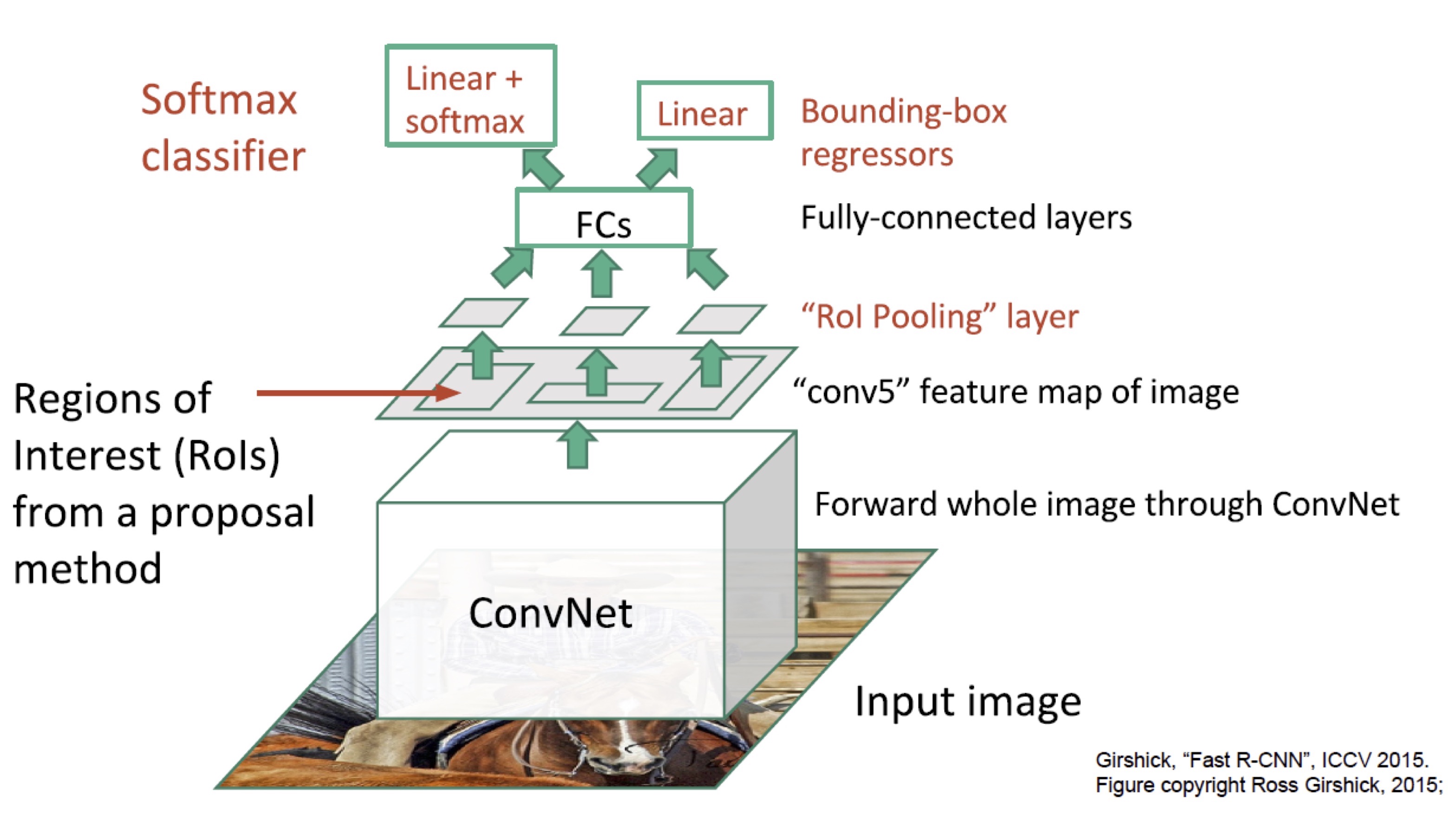
i. Apply CNN to An Entire Image
In this step, it applies ConvNet to an entire image, rather than each region of interest as R-CNN does, to produce a convolutional feature map
ii. Extract Feature Maps for Region Proposals
It extracts region proposals as done by R-CNN and projects these proposals onto the convolutional feature map. To fit the following FC layer, it employs a region of interest (RoI) pooling layer to convert these proposals into a fixed-length feature vector
The RoI Pooling Layer
Suppose that the original RoI has spatial size \( h\times w \), we want to obtain the resultant feature maps of size \( H\times W \)(e.g., \( 7\times 7 \)). The RoI pooling layer divides the original RoI into an \( H\times W \) grid of sub-window of approximate size \( h/H\times w/W \) and then max-pooling the values in each sub-window to obtain the resultant feature maps of size \( H\times W \). The last step is to concatenate these feature maps to form the feature vector of fixed length \( H\times W\times C \), where \( C \) is the number of channels
iii. Run Feature Vector through FC layers
It now runs the feature vector output by the RoI pooling layer through fully-connected layers, and then computes a multi-task loss which is comprised of two sub-losses: one is a log loss for classification and the other is a smooth \( L_1 \) loss for bounding-box regression.
The Smooth \( L1 \) loss
\[\begin{align} \mathrm{smooth}_{L1}(x) = \begin{cases} 0.5x^2&\mathrm{if}\ |x|<1\\\ |x|-0.5,& \mathrm{otherwise} \end{cases} \end{align}\]The smooth \( L_1 \) loss is less sensitive to outliers than the \( L_2 \) loss. When the regression target is unbounded, training with \( L_2 \) requires careful tuning of learning rates in order to prevent exploding gradients.
iv. Object Detection at Test Time
This step works almost the same as the detection step from R-CNN except that it scores the proposals via softmax cross entropy instead of SVMs.
Bottleneck
Fast R-CNN achieves near real-time rates when ignoring the time spent on region proposals. Now, proposal methods, such as selective search, become the computational bottleneck in the state-of-the-art detection systems.
Faster R-CNN
Faster R-CNN refines Fast R-CNN in that it generates proposals using a Region Proposal Network (RPN), which shares full-image convolutional features with the detection network, thus enabling nearly cost-free region proposals.
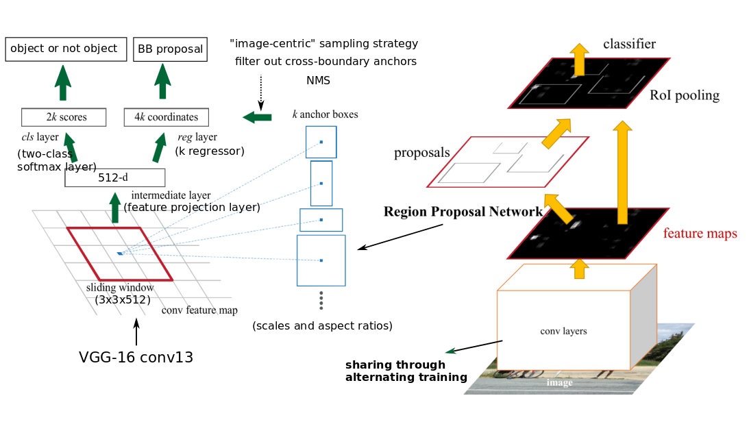
Region Proposal Network
The RPN built upon the shared convolutional layer consists of three convolutional layers—a \(3\times 3\) convolutional layer with 512 filters followed by two sibling \(1\times 1\) convolutional layers with \(4k\) and \(2k\) filters. We call the convolutional layer with \(4k\) filters the regression layer and the one with \(2k\) filters the classifier layer since the former produces adjustments to the coordinates of the \(k\) anchor boxes while the latter produces scores that estimate the probability of an object or not in each anchor. The RPN slides over the convolutional feature map produced by the shared convolutional layer, computing adjustments and objectness scores.
Output of RPN
At each location, the regression layer simultaneously outputs \( 4k \) adjustments to the coordinates of \( k \) anchor boxes, differing in scale and aspect ratio. The classifier layer produces \( 2k \) scores that estimate the probability of an object or not for each anchor.
Training and Loss Functions for RPN
-
The output feature map consists of about 40 x 60 locations, corresponding to 40609 ~ 20k anchors in total. At train time, all the anchors that cross the boundary are ignored so that they do not contribute to the loss. This leaves about 6k anchors per image.
-
An anchor is considered to be a “positive” sample if it satisfies either of the two conditions — a) The anchor has the highest IoU (Intersection over Union, a measure of overlap) with a groundtruth box; b) The anchor has an IoU greater than 0.7 with any groundtruth box. The same groundtruth box can cause multiple anchors to be assigned positive labels.
-
An anchor is labeled “negative” if its IoU with all groundtruth boxes is less than 0.3. The remaining anchors (neither positive nor negative) are disregarded for RPN training.
-
Each mini-batch for training the RPN comes from a single image. Sampling all the anchors from this image would bias the learning process toward negative samples, and so 128 positive and 128 negative samples are randomly selected to form the batch, padding with additional negative samples if there are an insufficient number of positives.
-
The training loss for the RPN is also a multi-task loss, given by
where \( L_{cls} \) is a log loss for objectness classification, and \( L_{reg} \) is a smooth \( L_1 \) loss for bounding-box regression identical to the regression loss defined in Fast R-CNN
Sharing Convolutional Features for RPN and Fast R-CNN
Sharing convolutional features is not as easy as simply define a single network that includes both RPN and Fast R-CNN, and then optimizing it jointly with back-propagation. The reason is that Fast R-CNN training depends on fixed region proposals and it is not clear a priori if learning Fast R-CNN will converge while simultaneously changing the proposal mechanism.
The authors develop a 4-step training algorithm to learn shared features via alternating optimization
- Train the RPN as described above. This network is initialized with ImageNet-pre-trained model and fine-tuned end-to-end for the region proposal task
- Train the Fast R-CNN using the proposals generated by the step-1 RPN. This detection network is also initialized by the ImageNet-pre-trained model. At this point, the two networks don’t share convolutional layers
- Use the detection network to initialize RPN training, but fix the shared convolutional layers and only fine-tune the layers unique to RPN. Now the two network share convolutional layers
- Keep the shared convolutional layers fixed, fine-tune the fc layers of Fast R-CNN
Filtering
To reduce redundancy, we apply non-maximum suppression with IoU threshold \( 0.7 \) on the proposal regions based on their objectness score. That is, if two proposals have more than \( 0.7 \) IoU with each other, we suppress the one with lower object score.
Advantages
An important property of the RPN is that it’s translation invariant, while k-mean clustering method used in YOLO is not.
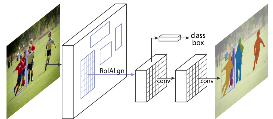
Mask R-CNN
Mask R-CNN extends Faster R-CNN, trying to do instance segmentation by adding a branch for predicting an object mask in parallel with the existing branch for bounding box recognition. The following figure illustrates the branch for instance segmentation.
There are two things noteworthy:
- Mask R-CNN resorts to an operation called RoIAlign rather than RoIPool for extracting a small feature map from each RoI
- The branch for instance segmentation is a fully convolutional network.
Here are some details about Mask R-CNN
RoIAlign
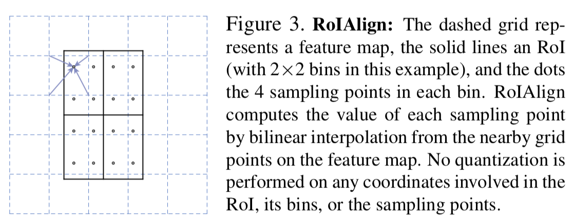
RoIPool is designed for object detection but not for semantic segmentation in that it performs quantization (i.e., rounds projected RoIs on the feature map and bins into which the RoIs is divided to produce input data for the next convolutional layer), thereby introducing misalignments.
The authors propose an RoIAlign layer that removes the harsh quantization of RoIPool, properly aligning the extracted features with the input. It simply omits any quantization of RoI boundaries or bins,
-
using bilinear interpolation to compute the exact values of the input features at \( 4 \) (or even \( 1 \) could make do) regularly sampled locations in each RoI bin
</figure>
- aggregating the result of each bin (using max or average)
Loss
The last convolutional layer of the mask branch is of size \( m\times m\times K \) where each of \( K \) binary channels encodes a class. The authors also suggest that a sigmoid for each class outperforms a softmax over all classes since the former one eases the competition among classes
With these in mind, now we define the loss for the mask branch on positive RoIs as below
\[\begin{align} L_{loss}={1\over m^2}\sum_{i=1}^m\sum_{j=1}^m\sigma(X_{i,j}[{y_{i,j}}]) \end{align}\]Where \( y_{i,j} \) is the label at position \( (i, j) \) and \( \sigma(X_{i,j}[y_{i,j}]) \) is the probability that position \( (i,j) \) is predicted to be \( y_{i,j} \). Furthermore, the label is determined by the intersection between an RoI and its associated ground-truth mask.
Inference
The inference is comprised of the following steps:
- Extract region proposals through RPN
- Run the box prediction branch on these proposals, followed by non-maximum suppression
- The mask branch is then applied to the highest scoring 100 detection boxes
- The \( m\times m\) floating-number mask output is then resized to the RoI size, and binarized at a threshold of \( 0.5 \)
Human Pose Estimation
One extension to Mask R-CNN is to use it for human pose estimation. To do so, we reuse the \( m \times m \) output of the mask branch. This time, we want to predict \( K \) keypoint types (e.g., left shoulder, right elbow). For each keypoint type, we define the training target as a one-hot \( m\times m \) binary mask where only a single point is labeled positive. During training, for each visible ground-truth keypoint, we minimize the cross-entropy over an \( m^2 \)-way softmax output. Note that we treat keypoint type independently as in instance segmentation
Summary
In this post, we briefly introduce a series of region-based methods for object detection, from R-CNN to Faster R-CNN. At last, we see how Mask R-CNN extends Faster R-CNN for instance segmentation.
Main Reference
Pedro F. Felzenszwalb and Daniel P. Huttenlocher. Efficient Graph-based Image Segmentation, Felzenszwalb and Huttenlocher
J. Uijlings, K. van de Sande, T. Gevers, and A. Smeulders. Selective search for object recognition
Ross Girshick, Jeff Donahue, Trevor Darrell, and Jitendra Malik. Rich feature hierarchies for accurate object detection and semantic segmentation
S. Ren, K. He, R. Girshick, and J. Sun. Faster R-CNN: Towards real-time object detection with region proposal net-works
Kaiming He, Georgia Gkioxari, Piotr Dollar, Ross Girshick. Mask R-CNN
https://towardsdatascience.com/faster-r-cnn-for-object-detection-a-technical-summary-474c5b857b46