
Introduction
Much ink has been spilled on MAML in our previous posts[1], [2]. In this post, we extend the topic to its application in reinforcement learning with nonstationary and competitive environments. Long story short, we cast the problem of continuous adaptation to a non-stationary task into the learning-to-learn framework, and resolve it through MAML.
In the rest of this post, we first review MAML-RL[1] introduced in the original MAML paper. Then we encode MAML-RL into a probablistic graphical model, and introduce our new problem setting. At last, we address this problem using a variant of MAML, introduced by Al-Shedivat et al. 2018.
TL; DR
To learn an adaptive RL method, Adaptive MARL assumes there is an underlying transition dynamics of the task distribution and modifies MAML so that the updated model samples trajectories from the next task(instead of the same task done in MAML). Moreover, it learns the adaptive step size through the outer loop learning.
MAML-RL
We only do a minimum review here for better comparison with the algorithm introduced later. The loss function of MAML-RL is defined as
\[\begin{align} \min_\theta &\sum_{T_i\sim p(T)}\mathcal L_{T_i}(\theta)\tag{1}\\\ where\quad \mathcal L_{T_i}(\theta):=&\mathbb E_{\tau_\theta^{1:K}\sim p_{T_i}(\tau|\theta)}\big[\mathbb E_{\tau_{\phi}\sim p_{T_i}(\tau|\phi)}[\mathcal L_{T_i}(\tau_\phi|\tau_{\theta}^{1:K},\theta)]\big]\\\ \phi=&\theta-\alpha\nabla_\theta\mathcal L_{T_i}(\theta)\tag{2} \end{align}\]where \(L_T\) is the negative of the reward collected along trajectory \(\tau_\phi\), and inner update step Eq.\((2)\) can be repeated multiple times if desirable.
Note that the above loss is in fact from E-MAML, proposed by Stadie et al. to directly account for the fact that \(\pi_\theta\) will impact the final returns \(R(\tau_\phi)\) by influencing the initial update Eq.\((2)\). We use this loss here only for better comparison with the algorithm we will introduce later. For more information, we refer the interested reader to our next post.
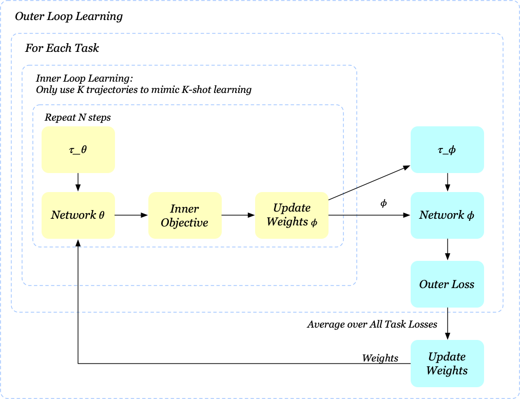
We now present the pseudocode of MAML-RL
\[\begin{align} &\mathbf{Algorithm\ MAML\_RL}\\\ 1.&\quad\mathrm{randomly\ initialize}\ \theta\\\ 2.&\quad\mathbf{while\ }not\ done\ \mathbf{do}\\\ 3.&\quad\quad\mathrm{sample\ a\ batch\ of\ tasks\ }T_{i}\sim p(T)\\\ 4.&\quad\quad\mathbf{for\ all\ }T_i\ in\ batch\ \mathbf{do}\\\ 5.&\quad\quad\quad\mathrm{sample\ }K\ \mathrm{trajectories\ }\tau_\theta^{1:K}\ \mathrm{using\ }\pi_\theta\\\ 6.&\quad\quad\quad\mathrm{compute}\ \phi=\phi(\tau_\theta^{1:K},\theta)\ \mathrm{as\ given\ in\ Eq}.(2)\\\ 7.&\quad\quad\quad\mathrm{sample\ trajectory\ }\tau_{\phi}\ \mathrm{using\ }\pi_\phi\\\ 8.&\quad\quad\mathbf{end\ for}\\\ 9.&\quad\quad\mathrm{minimize\ Eq}.(1)\ \mathrm{\ w.r.t. \theta\ using\ }\tau_{\phi}\ \mathrm{collected\ in\ step\ (7)}\\\ 10.&\quad\mathbf{end\ while} \end{align}\]We also visualize the training process
Problem Description
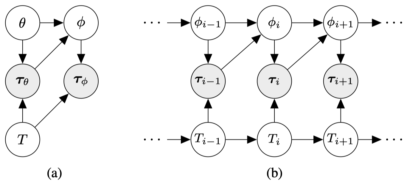
We can model MAML-RL as a probabilistic graphical model as \((a)\) shows, where \(\theta\) and \(\phi\) denote policy parameters, task variable \(T\) is sampled from a task distribution \(p(T)\), trajectory variables \(\tau_\theta\) and \(\tau_\phi\) are generated by following policy \(\pi_\theta\) and \(\pi_\phi\), respectively.
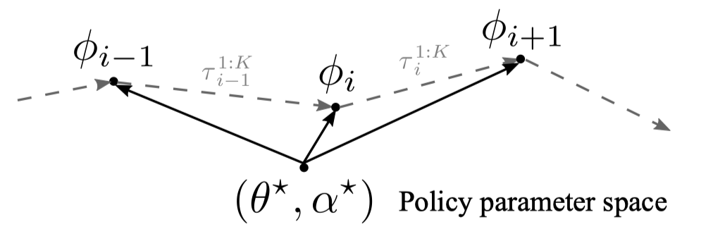
Now let’s consider a task changing dynamically due to non-stationary of the environment. We address this problem using a temporal probabilistic graphical model \((b)\), where \(T_{i}\) and \(T_{i+1}\) are sequentially dependent on transition distribution \(P(T_{i+1}\vert T_i)\). To adapt for task shift, we aim to learn policy parameter \(\theta\) and meta-learning rate parameter \(\alpha\) such that \(\theta\) can quickly adapt to task \(T_{i+1}\) from \(\tau_{i}^{1:K}\) within few gradient steps with step size \(\alpha\). The following figure illustrates this process.
MAML for Nonstationary Environments
Meta-Learning at Training Time
To train a model that adapts fast to \(T_{i+1}\) from \(\tau_{i}^{1:K}\) within few gradient steps, we define a loss similar to MAML-RL
\[\begin{align} \min_\theta &\mathbb E_{p(T_0),p(T_{i+1}|T_i)}\left[\mathcal \sum_{i=1}^L\mathcal L_{T_i,T_{i+1}}(\phi)\right]\tag{3}\\\ where\quad \mathcal L_{T_i,T_{i+1}}(\phi):=&\mathbb E_{\tau_{i,\theta}^{1:K}\sim p_{T_i}(\tau|\theta)}\big[\mathbb E_{\tau_{i+1,\phi}\sim p_{T_{i+1}}(\tau|\phi)}[\mathcal L_{T_{i+1}}(\tau_{i+1,\phi})|\tau_{i,\theta}^{1:K},\theta]\big]\\\ \phi=&\theta-\alpha\nabla_\theta\mathcal L_{T_i}(\theta)\tag{4} \end{align}\]Regardless of some changes of notations, the major distinction between Eq.\((3)\) and Eq.\((1)\) is that we now run policy \(\pi_\phi\) in the next task \(T_{i+1}\), which addresses our attempt on fast adaptation to \(T_{i+1}\). In deed, Eq.\((3)\) equally says that we want to learn an internal structure \(\theta\) such that after taking few gradient steps using trajectories \(\tau_{i,\theta}^{1:K}\), we wish it behave well in \(T_{i+1}\). The training process of our new method is similar to MAML-RL:
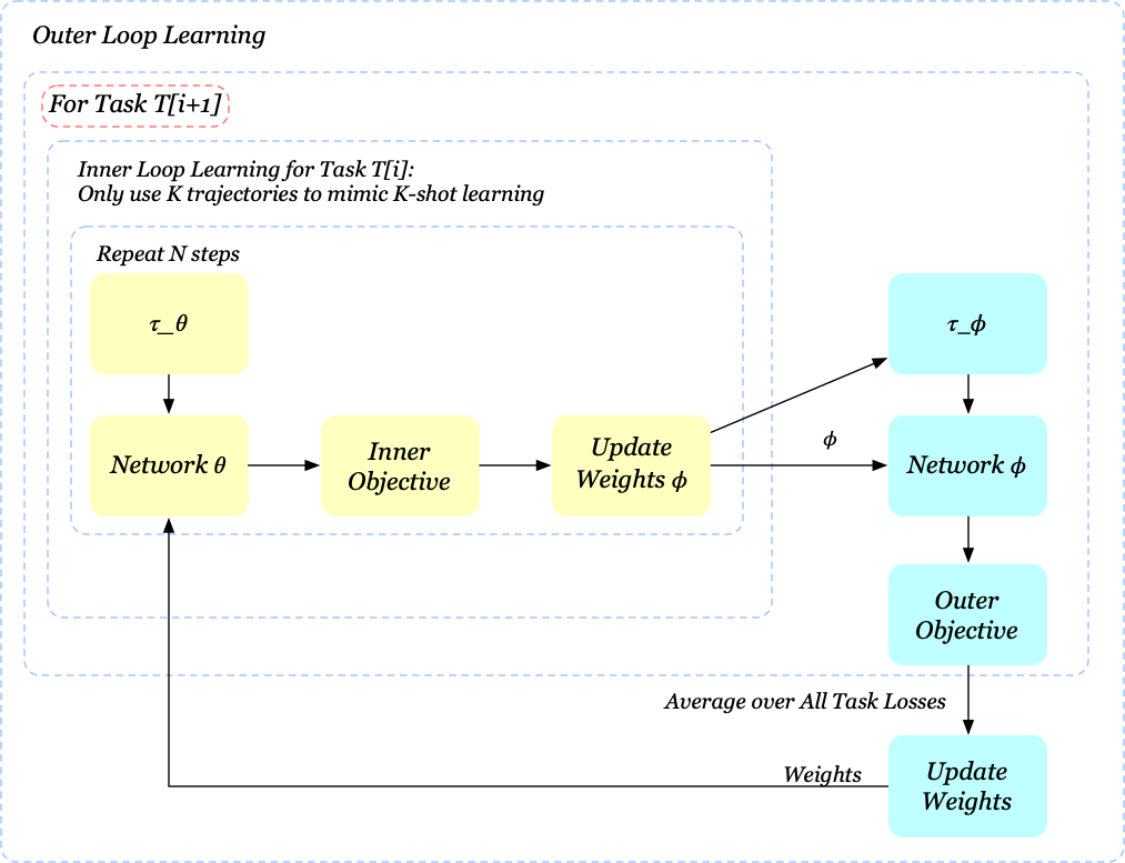
\[\begin{align} &\mathbf{Algorithm\ Meta\_Learning\_at\_training\_time}\\\ 1.&\quad\mathrm{randomly\ initialize}\ \theta, \alpha\\\ 2.&\quad\mathbf{while\ }not\ done\ \mathbf{do}\\\ 3.&\quad\quad\mathrm{sample\ a\ batch\ of\ task\ pairs\ }\{(T_{i},T_{i+1})\}_{i=1}^n\\\ 4.&\quad\quad\mathbf{for\ all\ }(T_i, T_{i+1})\ in\ batch\ \mathbf{do}\\\ 5.&\quad\quad\quad\mathrm{sample\ }K\ \mathrm{trajectories\ }\tau_\theta^{1:K}\ \mathrm{from\ }T_i\ \mathrm{using\ }\pi_\theta\\\ 6.&\quad\quad\quad\mathrm{compute}\ \phi=\phi(\tau_\theta^{1:K},\theta)\ \mathrm{as\ given\ in\ Eq}.(4)\\\ 7.&\quad\quad\quad\mathrm{sample\ trajectory\ }\tau_{\phi}\ \mathrm{from\ }T_{i+1}\ \mathrm{using\ }\pi_\phi\\\ 8.&\quad\quad\mathbf{end\ for}\\\ 9.&\quad\quad\mathrm{minimize\ Eq}.(3)\ \mathrm{\ w.r.t. \theta, \alpha\ using\ }\tau_{\phi}\ \mathrm{collected\ in\ step\ (7)}\\\ 10.&\quad\mathbf{end\ while} \end{align}\]We list two main differences between adaptive MAML and MAML-RL:
- For the purpose of adaptation, we sample pairs of sequential tasks in step 3 and sample trajectoreis from \(T_{i+1}\) in step 7.
- We additionally train the learning rate \(\alpha\) for each gradient step. This idea, originally proposed by Li et al. 2017 and further explored by Antoniou et al. 2019, has been demonstrated to improve the generalization performance in practice.
We also visualize the training process as before
Adaptation at Execution Time
Note that to compute unbiased adaptation gradients at training time, the agent runs policy \(\pi_\theta\) in \(T_i\) multiple times to collect \(K\) trajectories. Here, policy \(\pi_\theta\) does not necessarily optimize for maximal reward during training. At test time, however, the agent should maximize the total rewards, and thus it has to keep acting according to updated policy \(\pi_{\phi_i}\) in \(T_i\). To adjust for policy shift, we apply importance weight correction. Assuming the environment changes after every episode, we have
\[\begin{align} \phi_{i+1}:=\theta-\alpha{1\over K}\sum_{k=1}^K{\pi_\theta(\tau^k)\over\pi_{\phi_{k}}(\tau^k)}\nabla_{\theta}L_{T_{k}}(\tau^k)\tag{5} \end{align}\]where \(\pi_{\phi_k}\) is the policy used to collect \(\tau^k\) in task \(T_k\). In practice, we generally use the last \(K\) trajectories \(\tau^{1:K}_{i,\phi}\) to compute the new policy parameter.
The adaptation process is described in the following pseudocode
\[\begin{align} &\mathbf{Algorithm\ Adaptation\_at\_execution\_time}\\\ 1.&\quad\mathrm{initialize}\ \phi=\theta^\*\\\ 2.&\quad\mathbf{while\ }there\ are\ new\ incoming\ tasks\ \mathbf{do}\\\ 3.&\quad\quad\mathrm{get\ a\ new\ task\ }T_{i}\ \mathrm{from\ the\ stream}\\\ 4.&\quad\quad\mathrm{solve\ }T_{i}\ \mathrm{using\ policy\ }\pi_\phi,\ \mathrm{and\ collect\ trajectory\ }\tau\\\ 5.&\quad\quad\mathrm{update\ }\phi\leftarrow\phi(\tau^{1:K}_{i,\phi},\theta^\*, \alpha^\*)\ \mathrm{as\ given\ in\ Eq.}(5)\\\ 6.&\quad\mathbf{end\ while} \end{align}\]Experimental Results
We skip some outstanding results(which you may find here) and only illustrate one particular interesting below
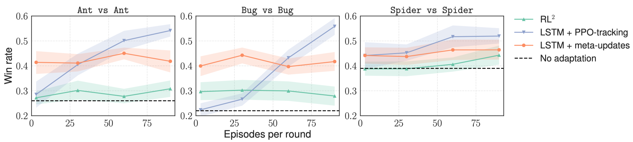
This figure illustrates the changes of winning rate versus episodes of gathered experience in test time; the red line shows the result of adaptive MAML combined with LSTM. As the number of episodes increase, the performance of our meta-learned strategy stays nearly constantly, while LSTM+PPO-tracking turns into “learning at test time” and slowly learn to compete against its opponent. This suggests that the meta-learned strategy acquires a particular bias at training time that allows it to perform better from limited experience but also limits its capacity of utilizing more data at test time.
References
- Maruan Al-Shedivat, Trapit Bansal, Yura Burda, Ilya Sutskever, Igor Mordatch, and Pieter Abbeel. Continuous Adaptation via Meta-Learning in Nonstationary and Competitive Environments
- Chelsea Finn, Pieter Abbeel, Sergey Levine. Model-Agnostic Meta-Learning for Fast Adaptation of Deep Networks
- Bradly C. Stadie, Ge Yang, Rein Houthooft, Xi Chen, Yan Duan, Yuhuai Wu, Pieter Abbeel, Ilya Sutskever. Some Considerations on Learning to Explore via Meta-Reinforcement Learning
- Jonas Rothfuss, Dennis Lee, Ignasi Clavera, Tamim Asfour, and Pieter Abbeel. ProMP: Proximal Meta-Policy Search. In ICLR 2019.
- Antreas Antoniou, Harrison Edwards, and Amos Storkey. How To Train Your MAML. in ICIR 2019
- Zhenguo Li, Fengwei Zhou, Fei Chen, and Hang Li. Meta-sgd: Learning to learn quickly for few shot learning.