
Introduction
Energy-based regularization has previously shown to improve both exploration and robustness in changing sequential decision-making tasks. It does so by encouraging policies to spread probability mass on all actions equally. However, entropy regularization might be undesirable when actions have significantly different importance. For example, some actions may be useless in certain tasks and uniform actions in this case would introduce fruitless exploration. Jordi Grau-Moya et al. 2019 propose a novel regularization that dynamically weights the importance of actions(i.e. adjusts the action prior) using mutual information.
Derivation of Mutual-Information Regularization
In the previous post, we framed the reinforcement learning problem as an inference problem and obtain the soft optimal objective as follows
\[\begin{align} \max_{\pi_0,\pi}\mathcal J(\pi_0, \pi)=\sum_{t=1}^T\gamma^{t-1}\mathbb E_{s_{t}, a_{t}\sim \pi}\left[r(s_t,a_t)-\tau\log{\pi(a_t|s_t)\over \pi_0(a_t)}\right]\tag{1} \end{align}\]where \(\tau\) is the temperature, \(\pi(a_t\vert s_t)\) is the action distribution of the policy to optimize, and the action prior \(\pi_0(a_t)\) is put back since we no longer assume it’s a uniform distribution here. Moving the expectation inward, we obtain
\[\begin{align} \max_{\pi_0,\pi}\mathcal J(\pi_0,\pi)=&\sum_{t=1}^T\gamma^{t-1}\left\{\mathbb E_{s_{t}, a_{t}\sim \pi}\left[r(s_t,a_t)\right]-\tau\mathbb E_{s_{t}, a_{t}\sim \pi}\left[\log{\pi(a_t|s_t)\over \pi_0(a_t)}\right]\right\}\\\ =&\sum_{t=1}^T\gamma^{t-1}\left\{\mathbb E_{s_{t}, a_{t}\sim \pi}\left[r(s_t,a_t)\right]-\tau\sum_{s_t} \pi(s_t)D_{KL}(\pi(a|s_t)\Vert \pi_0(a))\right\}\\\ =&\sum_{t=1}^T\gamma^{t-1}\mathbb E_{s_{t}, a_{t}\sim \pi}\left[r(s_t,a_t)\right]-\tau\sum_s\pi(s)D_{KL}(\pi(a|s)\Vert \pi_0(a))\tag{2}\\\ \Longrightarrow\max_\pi\mathcal J(\pi)=&\sum_{t=1}^T\gamma^{t-1}\mathbb E_{s_{t}, a_{t}\sim \pi}\left[r(s_t,a_t)\right]-\tau I_{\pi}(S;A)\tag{3}\\\ where\quad \pi(s)=&{1\over Z}\sum_{t=1}^T\gamma^{t-1}\sum_{s_t}\pi(s_t)\tag{4}\\\ =&{1\over Z}\sum_{t=1}^T\gamma^{t-1}\sum_{s_1,a_1,\dots,s_{t-1},a_{t-1}}\pi(s_1)\left(\prod_{t'=0}^{t-2}\pi(a_t'|s_t')P(s_{t'+1}|s_{t'},a_{t'})\right)\pi(a_{t-1}|s_{t-1})P(s|s_{t-1},a_{t-1}) \end{align}\]Here, \(\pi(s)\) is the discounted marginal distribution over states. We kind of abuse the equality sign in Equation \((2)\) as we implicitly add the partition function \(1\over Z\) to \(\pi(s)\). This, however, does not change our optimization objective since it’s a constant and can easily be corrected through \(\tau\).
From Equation \((2)\), we can see that maximizing \(\mathcal J(\pi_0,\pi)\) w.r.t. \(\pi_0\) equally minimizes \(\sum_sq(s)D_{KL}(\pi(a\vert s)\Vert \pi_0(a))\), which is minimized when \(\pi_0(a)=\pi(a)\):
\[\begin{align} &\pi(s)D_{KL}(\pi(a|s)\Vert \pi_0(a)) - \pi(s)D(\pi(a|s)\Vert \pi(a))\\\ =&\sum_{s,a}\pi(s,a)\left(\log{\pi(a|s)\over \pi_0(a)}-\log {\pi(a|s)\over \pi(a)}\right)\\\ =&\sum_{s,a}\pi(s,a)\log{\pi(a)\over \pi_0(a)}\\\ =&\sum_{a}\pi(a)\log{\pi(a)\over \pi_0(a)}\\\ =&D_{KL}(\pi\Vert \pi_0)\ge0 \end{align}\]Therefore, we can derive Equation \((3)\) by substitute \(\pi\) for \(\pi_0\) in Equation \((2)\).
Equation.\((3)\) suggests that when the action distribution of the current policy is taken as the action prior, our soft optimal objective now penalizes the mutual information between state and action. Intuitively, this means that we want to discard information in \(s\) irrelevant to the agent’s performance.
With the form of the optimal prior for a fixed policy at hand, one can easily devise a stochastic approximation method (e.g. \(\pi_0(a)=(1-\alpha)\pi_0(a)+\alpha \pi(a\vert s)\) with \(\alpha\in[0,1]\) and \(s\sim \pi(s)\)) to estimate the optimal prior \(\pi_0(a)\) from the current estimate of the optimal policy \(\pi(a\vert s)\).
Mutual Information Reinforcement Learning Algorithm
Now we apply mutual information regularization to deep \(Q\)-networks(DQN). The algorithm, Mutual Information Reinforcement Learning(MIRL), makes five updates to traditional DQN:
Initial Prior Policy: For an initial fixed policy \(\pi(a\vert s)\), we compute \(\pi_0(a)\) by minimizing \(\sum_{s}\pi(s)D_{KL}(\pi(a\vert s)\Vert \pi_0(a))\).
Prior Update: We approximate the optimal prior by employing the following update equation
\[\begin{align} \pi_0(a)=(1-\alpha_{\pi_0})\pi_0(a)+\alpha_{\pi_0} \pi(a|s) \end{align}\]where \(s\sim \pi(s)\) and \(\alpha_{\pi_0}\) is the step size.
\(Q\)-function Updates: Concurrently to learning the prior, MIRL optimizes \(Q\)-function by minimizing the following loss
\[\begin{align} L(\theta)&:=\mathbb E_{s,a,r,s'\sim replay}\left[\left(\mathcal T_{soft}^{\pi_0}Q^{-}(s,a,s')-\pi(s,a)\right)^2\right]\tag {13}\\\ where\quad (\mathcal T_{soft}^{\pi_0}Q)(s,a,s')&:=r(s,a)+\gamma{\tau}\log\sum_{a'}\pi_0(a')\exp( Q^-(s',a')/\tau) \end{align}\]where \(Q^-\) denotes the target \(Q\)-function
Behavioral Policy: MIRL’s behavioral policy consists of two parts: when exploiting, it takes greedy action based on the soft optimal policy; when exploring, it follows the optimal prior distribution. Mathematically, given a random sample \(u\sim \mathrm{Uniform}[0,1]\) and epsilon \(\epsilon\), the action is obtained by
\[\begin{align} a= \begin{cases} \arg\max_a\pi(a|s)&\mathrm{if}\ u>\epsilon\\\ a\sim \pi_0(\cdot)&\mathrm{if}\ u\le\epsilon \end{cases}\\\ where\quad \pi(a|s)={1\over Z}\pi_0(a)\exp(\pi(s,a)/\tau) \end{align}\]\(\tau\) Update: the temperature \(\tau\) controls penalty for the mutual information between state and action. As one might expect, it should be large at first and gradually anneals down during training process to ensure initial exploration. MIRL updates the inverse of \(\tau\), \(\beta={1\over\tau}\), according to the inverse of the empirical loss of the \(Q\)-function
\[\begin{align} \beta=(1-\alpha_\beta)\beta+\alpha_{\beta}\left({1\over L(\theta)}\right) \end{align}\]where \(\alpha_\beta\) is the step size. The intuition is that we want \(\tau\) to be large when the loss of the \(Q\)-function is large. Note that a large \(Q\)-function loss stems from either inaccurate estimate of \(Q\) or large \(Q\)-values. Both cases makes sense of a large \(\tau\). However, regarding the different scale of \(\tau\) and \(L(\theta)\), an additional multiplier may be desirable.
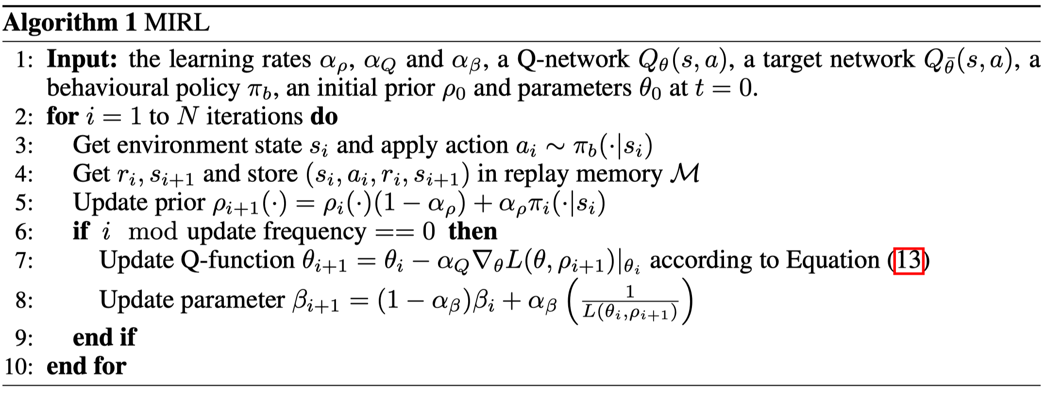
Algorithm
Now it is straightforward to see the whole algorithm
References
Grau-Moya, Jordi, Felix Leibfried, and Vrancx Peter. 2019. “Soft \pi-Learning with Mutual-Information Regularization.” ICLR 2019, 1–9.