
Introduction
In our previous post, we discussed Transformer, an architecture that utilizes self-attention for sequential modeling/entity selection. Transformer has been successfully applied in NLP, CV and RL, demostrating its versatility in many cases. Despite all these success, one major limitation of Transformer is that it is only applicable to fixed-length context. In this post, we discuss a novel architecture called TransformerXL(mea ning extra long), proposed by Day&Yang et al. 2019, that extends Transformer beyond a fixed length without discrupting temporal coherence.
Preliminaries
In this section, we briefly review the Transformer architecture. Figure 1 gives us an overview of the transformer architecture, which consists of an encoder and a decoder.
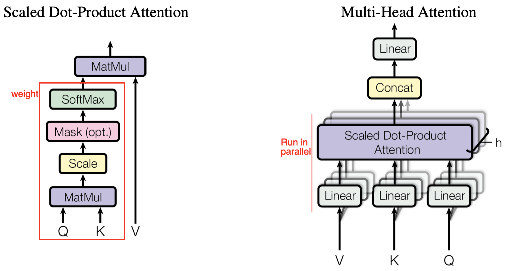
Encoder: The encoder comprises a stack of identity layers. Each layer has two sub-layers. The first is a multi-head self-attention mechanism(Figure 2(right)), and the second is a simple feed forward network. Residual connections are employed around as shown in the figure.
Decoder: The decoder is also composed of a stack of identity layers. Each layer has three sub-layers. The first is a masked multi-head self-attention mechanism, where the mask is used to prevent attention to out-of-sequence positions. The second multi-head self-attention mechanism, taking keys and values from the encoder, performs attention over the output of the encoder stack. The third is simply a feed forward network as in the encoder. Residual connections are employed around as in the encoder.
We formally define the multi-head self-attention mechanism as follows
\[\begin{align} \pmb q,\pmb k,\pmb v&=\pmb xW_Q,\pmb xW_K,\pmb xW_V\\\ \alpha_{hqk}&=\text{einsum}(\pmb q_{hqd},\pmb k_{hkd})\\\ \pmb w_{hqk}&=\text{MaskedSoftmax}(\alpha_{hqk})\\\ \pmb y_{hqk}&=\text{einsum}(\pmb w_{hqk},\pmb v_{hkd})\\\ \pmb y &=\pmb x+\pmb y_{hqk}W_Y\\\ \pmb y&=\text{LayerNorm}(\pmb y) \end{align}\tag {1}\]where \(\pmb x\) is the input and we use Einstein summation to denote the tensor multiplication.
Since the self-attention mechanism and feed forward network themselves do not bear any sequential information, an additional positional encoding is added to the input embeddings of both the encoder and decoder to tip off the sequential orders. In Transformer, the positional encoding are encoded using the sine and cosine functions of different frequencies
\[\begin{align} \pmb p_{(pos, 2i)}&=\sin(pos/10000^{2i/d})\\\ \pmb p_{(pos, 2i+1)}&=\cos(pos/10000^{2i/d}) \end{align}\tag2\]where \(pos\) is the token’s absolute position in the current segment, \(i\) is the \(i\)-th dimension and \(d\) is dimension.
When applying Transformer to sequential modeling, a simple practice to avoid OOM is to divide sequences into shorter segments and only train the model within each segment, ignoring all contextual information from previous segments. This scheme raises several problems:
- It restricts the model to only attend to a fixed length of sequences, preventing capturing longer-term dependences.
- The fixed length segments are created by selecting a consecutive chunk of symbols without respecting any other semantic boundary. Hence, in some cases, the model may lack necessary contextual information needed to well predict the next symbol, leading to inefficient optimization and inferior performance. Dai et al refers to this problem as context fragmentation.
- During evaluation, at each step, it make predictions based on a whole segment of the same length as in training. Although this procedure ensures each prediction utilizes the longest possible context, it’s extremely expensive and inefficient as it frequently reevaluates previous contents (see Figure 3b).
TransformerXL
TransformerXL uses a similar structure as Transformer, with a few improvements. First, it caches and reuses the hidden state sequence computed from the previous segment. We discuss these improvements in details in this section
Segment-Level Recurrence with State Reuse
As shown in Figure 2(a), when training a new segment, we take into account the hidden states of the previous segment. These previous states are fixed and we do not propagate gradients to them. Allowing the current segment to take advantage of the previous states enables the network to model longer-term dependency beyond the fixed window and alleviates the context fragmentation issue.
Formally, let the two consecutive segments of length \(L\) be \(\pmb s_\tau\) and \(\pmb s_{\tau+1}\). Denote the \(n\)-th layer hidden state sequence of \(\pmb s_\tau\) by \(\pmb h_\tau^n\in\mathbb R^{L\times d}\), where \(L\) is the sequence length and \(d\) is the hidden dimension. Then, the \(n\)-th layer hidden state for segment \(\pmb s_{\tau+1}\) is produced as follows
\[\begin{align} \tilde {\pmb h}_{\tau+1}^{n-1}&=[\text{SG}(h_\tau^{n-1}),h_{\tau+1}^{n-1}]\\\ \pmb q_{\tau+1}^n, \pmb k_{\tau+1}^n, \pmb v_{\tau+1}^n&={\pmb h}_{\tau+1}^{n-1}W_q,\tilde {\pmb h}_{\tau+1}^{n-1}W_k, \tilde {\pmb h}_{\tau+1}^{n-1}W_v\\\ \pmb h_{\tau+1}^n&=\text{Transformer-Layer}(\pmb q_{\tau+1}^n, \pmb k_{\tau+1}^n, \pmb v_{\tau+1}^n) \end{align}\tag {3}\]where \(\text{SG}\) denotes stop-gradient, \([\pmb h_1,\pmb h_2]\) concatenates \(\pmb h_1\) and \(\pmb h_2\) along the sequential dimension.
Anothe benefit that comes with the recurrence scheme is significantly faster evaluation. We can reuse the previous segments instead of recompute them!
Finally, notice that the recurrence scheme does not need to be restricted to only the previous segment – it can use more than one previous segments as long as the GPU memory allows. In their experiments, they use the previous segment in training and extend to far before during evaluation. This is feasible as the recurrence scheme only changes the lengths of the key and value and leave the final hidden state \(\pmb h\) as it is.
Relative Positional Encodings
While the above idea is appealing, it comes with a crucial challenge. That is, how can we keep the positional information coherent when we reuse the states? The encoding method in the previous section fails since it uses the same position encoding for the previous and current segments. For example, a segment of length \(4\) encodes positions \([0, 1, 2, 3]\). Now we have two segments and both using the same positions \([0, 1, 2, 3]\) makes the semantics of positions incoherent, resulting in a sheer performance loss.
In order to avoid this failure mode, the fundamental idea is to only encode the relative positional information in the hidden states. As a result, Dai et al. propose a novel relative positional encoding, which not only has one-to-one correspondence to its absolute couterpart but also enjoys much better generalization empirically. First, we rewrite the standard attention score \(\alpha\), which previously computed using Einstein summation
\[\begin{align} \alpha_{ij}&=(\pmb x_i+\pmb p_i)W_qW_k^\top (\pmb x_j+\pmb p_j)\\\ &=\pmb x_iW_qW_k^\top \pmb x_j^\top+\pmb x_iW_qW_k^\top\pmb p_j^\top+\pmb p_iW_qW_k^\top\pmb x_j^\top+\pmb p_iW_qW_k^\top\pmb p_j^\top \end{align}\tag {4}\]where \(\pmb x\) and \(\pmb p\) are row vectors of their corresponding matrices. The newly proposed form with relative positional encodings is as follows
\[\begin{align} \alpha_{ij}=\underbrace{\pmb x_iW_q\color{blue}{W_{k,x}^\top} \pmb x_j^\top}_{a}+\underbrace{\pmb x_iW_q\color{green}{W_{k,r}^\top\pmb r_{i+M-j}^\top}}_{b}+\underbrace{\color{red}{\pmb u}\color{blue}{W_{k,x}^\top}\pmb x_j^\top}_{c}+\underbrace{\color{red}{\pmb v}\color{green}{W_{k,r}^\top\pmb r_{i+M-j}^\top}}_d{}\tag {5} \end{align}\]where \(\pmb u\) and \(\pmb v\) are row vectors, \(i\in{0,\dots,L-1}\) and \(j\in{0,\dots,M+L-1}\), and \(M\) and \(L\) are the cache and segment lengths, respectively. Unlike the original equation in the paper, we add \(M\) to the subscript of \(\pmb r\) to make things more clear.
We summarize changes as follows
- The first change is to replace all appearances of the absolute positional encoding \(\pmb p_j\) with its relative counterpart \(\pmb r_{i+M-j}\). Note that \(\pmb r\) is a sinusoid encoding as in Equation \((2)\).
- Secondly, the absolutely positional query vector \(\pmb p_iW_q\) is replaced by its relative counterpart, a trainable vector \(\pmb u\in \mathbb R^d\), since the positional query vector is the same for all query positions.
- Finally, we use two separate weight matrices \(W_{k, x}\) and \(W_{k,r}\) for producing the content-based key vectors and location-based key vectors respectively.
Under the new parameterization, each term has an intuitive meaning:
- (a) represents content-based addressing, the relative weights of \(\pmb k_j\) to \(\pmb q_i\)
- (b) captures a content-dependent positional bias, the relative positional weights of position \(j\) to \(\pmb q_i\)
- (c) governs a global content bias, the global weights of \(\pmb k_j\)
- (d) encodes a global positional bias, the global weights of position \(j\)
Reducing Computational Cost of Attention with Relative Positional Embedding
The naive way to compute \(\alpha\) require computing \(W^\top_{k,r}\pmb r^\top_{i+M-j}\) for all pairs \((i,j)\), whose cost is quadratic w.r.t. the sequence length. In this subsection, we reduce the cost to linear. First, notice that the relative distance \(i-j\) can only be integer from \(0\) to \(M+L-1\), where \(M\) is the cache length and \(L\) is the segment length. This allows us to compute all \(\pmb r W_{k,r}\) at once
\[\begin{align} \pmb q=\pmb r W_{k,r}= \begin{bmatrix} \pmb r_{M+L-1} W_{k,r}\\\ \pmb r_{M+L-2} W_{k,r}\\\ \vdots\\\ \pmb r_{0} W_{k,r} \end{bmatrix}\in\mathbb R^{(M+L)\times d} \end{align}\]Notice that we define \(\pmb q\) in a reversed order, i.e., \(\pmb q_i=\pmb r_{M+L-1-i}W_{k,r}\), to make further discussion easier.
We collect the term \((b)\) for all possible \((i,j)\) into the following \(L\times(M+L)\) matrix
\[\begin{align} \pmb b= \begin{bmatrix} \tilde {\pmb x}_0\pmb q_{L-1}^\top&\tilde {\pmb x}_0\pmb q^\top_{L}&\dots&\tilde {\pmb x}_{0}\pmb q^\top_{M+L-1}&0&\dots &0\\\ \tilde {\pmb x}_1\pmb q_{L-2}^\top&\tilde {\pmb x}_1\pmb q^\top_{L-1}&\dots&\tilde {\pmb x}_1\pmb q^\top_{M+L-2}&\tilde {\pmb x}_1\pmb q^\top_{M+L-1}&\dots &0\\\ \vdots&\vdots&\ddots&\vdots&\vdots&\ddots&\vdots\\\ \tilde {\pmb x}_{L-1}\pmb q_{0}^\top&\tilde {\pmb x}_{L-1}\pmb q^\top_{1}&\dots&\tilde {\pmb x}_{L-1}\pmb q^\top_{M+1}&\tilde {\pmb x}_{L-2}\pmb q^\top_{M+2}&\dots &\tilde {\pmb x}_{L-1}\pmb q^\top_{M+L-1}\\\ \end{bmatrix} \end{align}\]where \(\tilde {\pmb x}=\pmb xW_q\). Then we further define
\[\begin{align} \tilde{\pmb b}=\tilde{\pmb x}\pmb q^\top= \begin{bmatrix} \tilde {\pmb x}_0\pmb q_0^\top&\tilde {\pmb x}_0\pmb q^\top_{1}&\dots&\tilde {\pmb x}_0\pmb q^\top_{M+1}&\tilde {\pmb x}_0\pmb q^\top_{M+2}&\dots &\tilde {\pmb x}_0\pmb q^\top_{M+L-1}\\\ \tilde {\pmb x}_1\pmb q_0^\top&\tilde {\pmb x}_1\pmb q^\top_{1}&\dots&\tilde {\pmb x}_1\pmb q^\top_{M+1}&\tilde {\pmb x}_1\pmb q^\top_{M+2}&\dots &\tilde {\pmb x}_1\pmb q^\top_{M+L-1}\\\ \vdots&\vdots&\ddots&\vdots&\vdots&\ddots&\vdots\\\ \tilde {\pmb x}_{L-1}\pmb q_0^\top&\tilde {\pmb x}_{L-1}\pmb q^\top_{1}&\dots&\tilde {\pmb x}_{L-1}\pmb q^\top_{M+1}&\tilde {\pmb x}_{L-1}\pmb q^\top_{M+2}&\dots &\tilde {\pmb x}_{L-1}\pmb q^\top_{M+L-1}\\\ \end{bmatrix} \end{align}\]Now, it is easy to see that the \(i\)-th row of \(\pmb b\) is the result of shifting the \(i\)-th row of \( \tilde{\pmb b}\) by \(L-1-i\) positions.
Similarly, we can collect the term \(d\) for all possible \((i,j)\) into another \(L\times(M+L)\) matrix:
\[\begin{align} \pmb d= \begin{bmatrix} \pmb v\pmb q_{L-1}^\top&\pmb v\pmb q^\top_{L}&\dots&\pmb v\pmb q^\top_{M+L-1}&0&\dots &0\\\ \pmb v\pmb q_{L-2}^\top&\pmb v\pmb q^\top_{L-1}&\dots&\pmb v\pmb q^\top_{M+L-2}&\pmb v\pmb q^\top_{M+L-1}&\dots &0\\\ \vdots&\vdots&\ddots&\vdots&\vdots&\ddots&\vdots\\\ \pmb v\pmb q_{0}^\top&\pmb v\pmb q^\top_{1}&\dots&\pmb v\pmb q^\top_{M+1}&\pmb v\pmb q^\top_{M+2}&\dots &\pmb v\pmb q^\top_{M+L-1}\\\ \end{bmatrix} \end{align}\]Then we following the same procedure to define
\[\begin{align} \tilde{\pmb d}= \begin{bmatrix} \pmb v \pmb q_0&\pmb v \pmb q_1&\dots&\pmb v \pmb q_{M+1}&\pmb v \pmb q_{M+2}\dots\pmb v \pmb q_{M+L-1} \end{bmatrix} \end{align}\]Again, we can obtain \(\pmb d\) from \(\tilde{\pmb d}\) using a set of left-shift operations.
References
<a name=#ref1></a>Dai, Zihang, Zhilin Yang, Yiming Yang, Jaime Carbonell, Quoc V. Le, and Ruslan Salakhutdinov. 2020. “Transformer-XL: Attentive Language Models beyond a Fixed-Length Context.” ACL 2019 - 57th Annual Meeting of the Association for Computational Linguistics, Proceedings of the Conference, 2978–88. https://doi.org/10.18653/v1/p19-1285.
Code: https://github.com/kimiyoung/transformer-xl