
Introduction
This post talks about t-SNE, an unsupervised learning algorithm for embedding high-dimensional data in a low-dimensional space for visualization. We’ll first start from its predecessor, stochastic neighbor embedding (SNE), and then introduce t-SNE, seeing how t-SNE improves from SNE
Table of Contents
Stochastic Neighbor Embedding
Similarity
Define the similarity of datapoint \( x_j \) to datapoint \( x_i \) as the conditional probability density under a Gaussian centered at \( x_i \). Mathematically, the conditional probability \( p_{j\vert i} \) is given by
\[\begin{align} p_{j|i}={\exp(-\left|x_j-x_i\right|^2/2\sigma_i^2)\over\sum_{k\ne i}\exp(-\left|x_k-x_i\right|^2/2\sigma_i^2)} \end{align}\]where \( \sigma_i \) will be defined later.
We also define the similarity conditional probability of the counterparts \( y_j \) and \( y_i \) of \( x_j \) and \( x_i \) in the low-dimensional space, \( q_{j\vert i} \), as
\[\begin{align} q_{j|i}={\exp(-\left|y_j-y_i\right|^2)\over \sum_{k\ne i}\exp(-\left|y_k-y_i\right|^2)} \end{align}\]Loss Function
If the map points \( y_i \) and \( y_j \) correctly model the similarity between the high-dimensional datapoints \( x_i \) and \( x_j \), the conditional probabilities \( p_{j\vert i} \) and \( q_{j\vert i} \) will be equal. In light of that, SNE aims to find a low-dimensional map points that minimize the mismatch between \( p_{j\vert i} \) and \( q_{j\vert i} \). A natual measure of the faithfulness with which \( q_{j\vert i} \) models \( p_{j\vert i} \) is the Kullback-Leibler divergence. SNE tries to minimize the sum of KL divergences over all datapoints using a gradient descent method with momentum, in which the cost function \( C \) is defined by
\[\begin{align} C=\sum_iKL(P_i\vert|Q_i)=\sum_i\sum_jp_{j|i}\log{p_{j|i}\over q_{j|i}} \end{align}\]The gradient in paper is, (however I derived a more complex, different result:( )
\[\begin{align} {\partial C\over \partial y_i}=2\sum_j(y_i-y_j)(p_{j|i}-q_{j|i}+p_{i|j}-q_{j|i}) \end{align}\]I’ll leave the intuition behind this gradient later when we talk about t-SNE
Variance in Gaussian
The variance for a data point should be consistent with the density of the data so that the Gaussian can model the similarity properly. That is, it should be small in dense regions and large in sparse regions. SNE performs a binary search for the value of \( \sigma_i \) that produce a probability distribution \( P_i \) with a fixed perplexity that is specified by users. The perplexity is defined as
\[\begin{align} Perp(P_i) = 2^{H(P_i)}\tag {1} \end{align}\]where \( H(P_i) \) is the Shannon entropy of \( P_i \) measured in bits, defined as
\[\begin{align} H(P_i)=-\sum_jp_{j|i}\log_2 p_{j|i} \end{align}\]Since \( H(P_i) \) can be addressed as the minimum possible number of bits per message that would be needed (on average) to losslessly encode events drawn from \( P_i \), \( Perp(P_i) \) can be intuitively interpreted as a smooth measure of the effective number of neighbors
Drawbacks
- SNE resorts to adding Gaussian noise at the initial stage to help escape from local minima. It requires sensible tuning on the initial Gaussian and the rate at which it decays. These parameters, unfortunately, interact with learning rate and momentum used in gradient descent, which makes the optimization of SNE extremely hard
- It faces the crowding problem, which says that mapping high-dimensional data into low-dimensional space causes loss of distance information
t-SNE
Improvements from SNE
t-SNE differs from SNE in two ways:
- It uses joint probabilities instead of conditional probabilities to simplify gradients.
- It employs a heavy-tailed distribution in the low-dimensional space (in contrast with the Gaussian distribution in the high-dimensional space) to alleviate both the crowding problem and the optimization problems.
Similarity
In t-SNE, the joint probabilities in high-dimensional space are
\[\begin{align} p_{ij}={p_{i|j}+p_{j|i}\over 2n} \end{align}\]Where \( n \) is the number of data points. We’ll see later, \( n \) introduced in the divisor is to counteract the effect of the change of divisor in \( q_{ij} \).
On the other hand, we employ a Student t-distribution with one degree of freedom as the heavy-tailed distribution in the low-dimensional map. Using this distribution, the joint probabilities \( q_{ij} \) are defined as
\[\begin{align} q_{ij}={(1+\Vert y_i-y_j\Vert^2)^{-1}\over\sum_{k\ne l}(1+\Vert y_k-y_l\Vert^2)^{-1}}\tag {4} \end{align}\]Notice that the divisor is independent of \( i \) and \( j \), so there are \( n(n-1) \) multipliers. This is different from the number of multipliers in the divisor of \( p_{i\vert j} \) and \( p_{j\vert i} \), which is \( n-1 \)
Gradient
The gradient of the KL divergence between the two joint probabilities is then given by
\[\begin{align} {\partial C\over\partial y_i}=4\sum_j(y_i-y_j)(p_{ij}-q_{ij})(1+\Vert y_i-y_j\Vert^2)^{-1}\tag {5} \end{align}\]Thereby we have \( \Delta y_i \)
\[\begin{align} \Delta y_i &= -{\partial C\over \partial y_i}\\\ &=4\sum_j(y_j-y_i)(p_{ij}-q_{ij})(1+\Vert y_i-y_j\Vert^2)^{-1} \end{align}\]Now let’s drop the math for time being and get down to think what’s really going on behind this equation. The \( \Delta y_i \) says that, to a specific data point \( i \), if the similarity of it and its neighbor \( j \) in the map space is smaller than that in the original space (\( p_{ij}-q_{ij} > 0 \)), then \( j \) tries to draw \( i \) closer to it a little bit in the map space (\( (y_j-y_i) \) multiplies some positive). On the other hand, if the similarity of these two points in the map space is greater than that in the original space (\( p_{ij}-q_{ij} < 0 \)), then \( j \) tries to push \( i \) away a little bit (\( (y_j-y_i) \) multiplies some negative). The divisor \( 1+\Vert y_i-y_j\Vert^2 \) ensures the influence of \( j \) to \( i \) is weak when \( j \) is far away from \( i \) in the map space, and strong when close.
Algorithm
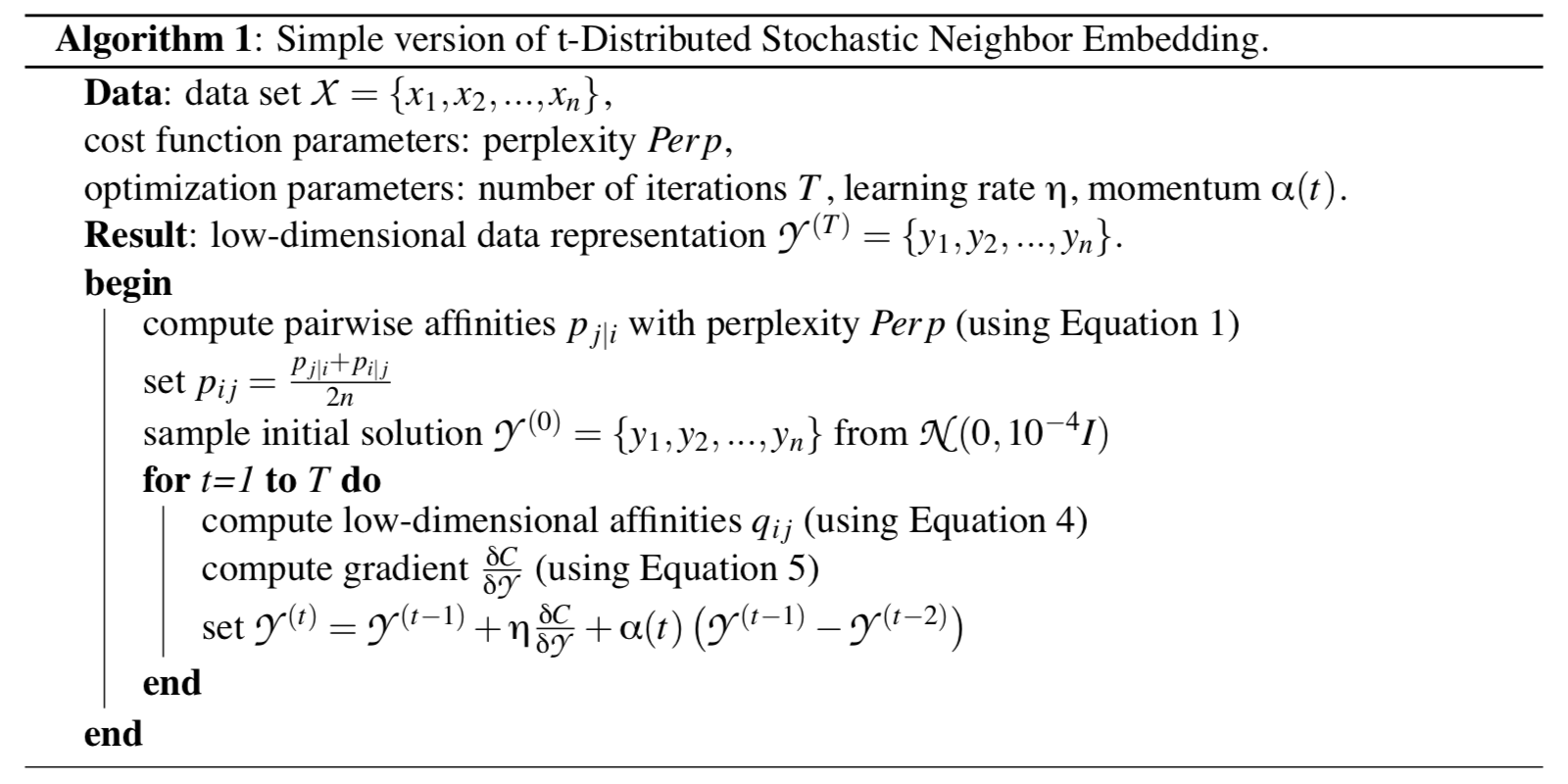
The equations in the algorithm are exactly those tagged in the previous part of this post. The algorithm also employs gradient descent with momentum to escape from local minima and accelerate the convergence of data points in the low-dimensional space.
References
https://distill.pub/2016/misread-tsne/#citation