Dreamer

Introduction

We discuss a model-based reinforcement learning agent called Dreamer, proposed by Hafner et al. 2020 in Google Brain, that achieves state-of-the-art performance on a variety of image-based control tasks but requires much fewer samples than the contemporary model-free methods.

Overview

Dreamer is composed of three parts:

Dynamics learning: Dreamer learns a dynamics model comprised of four components: a representation model \(p(s_t\vert s_{t-1},a_{t-1},o_t)\), a transition model \(q(s_t\vert s_{t-1}, a_{t-1})\), an observation model \(q(o_t\vert s_t)\), and a reward model \(q(r_t\vert s_t)\).
Behavior learning: Based on the dynamics model, Dreamer learns an actor-critic architecture, where the actor is denoted as \(q_\phi(a_t\vert s_t)\) and the value function is \(v_\psi(s_t)\).
Environment interaction: Dreamer interacts with the environment using the actor \(q(a_t\vert s_t)\) for data collection.

Dynamics Learning

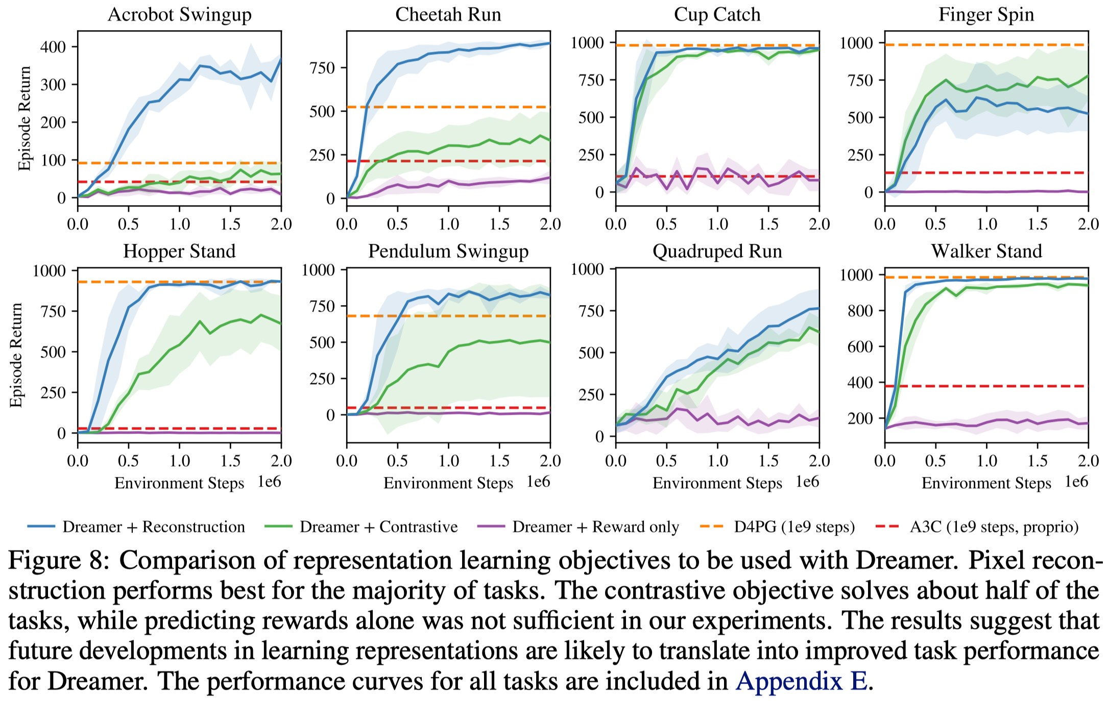
Hafner et al. experimented three approaches for learning representation: reward prediction, image reconstruction, and contrastive estimation. They found image reconstruction performs best in experiments, as shown in Figure 8. We next discuss the architecture used for image reconstruction, leaving the other two to Supplementary Materials for interested readers.

Architecture

Dreamer represents the dynamics as a sequential model with the following components

\[\begin{align} &\text{Representation model:}&p(s_t|s_{t-1},a_{t-1},o_t)\\\ &\text{Observation model:}&q(o_t|s_t)\\\ &\text{Reward model:}&q(r_t|s_t)\\\ &\text{Transition model:}&q(s_t|s_{t-1},a_{t-1}) \end{align}\]

where all models are parameterized by (de)convolutional/fully-connected networks with Gaussian heads. In the rest of the post, we refer to the transition model as the prior and the representation model as the posterior as the latter is additionally conditioned on the observation.

Figure 1. The recurrent state-space model(RSSM) in a single time step. When training the dynamics, the GRU takes the posterior stochastic state s' as the input. The output of the GRU is then passed to a hidden layer to produce parameters for the stochastic state distributions. Image embedding e_t is concatenated when computing the posterior. When training the actor-critic architecture, the GRU takes in the prior stochastic state s, and the posterior is not involved at all.

In practice, Dreamer uses the same architecture as its predecessor PlaNet, namely recurrent state-space model(RSSM), which splits the state space into stochastic and deterministic components(see Figure 1 left). This gives us the following models

\[\begin{align} &\text{Deterministic state model:}&h_t=f(h_{t-1},s_{t-1},a_{t-1})\\\ &\text{Prior Stochastic state model:}&s_t\sim q(s_t|h_t)\\\ &\text{Posterior Stochastic state model:}&s_t\sim p(s_t|h_t, e_t)\\\ &\text{Observation model:}&o_t\sim q(o_t|h_t,s_t)\\\ &\text{Reward model:}&r_t\sim q(r_t|h_t,s_t) \end{align}\]

where \(f\) is a recurrent neural network, e.g., a GRU

There are two notes you need to be aware of about RSSM:

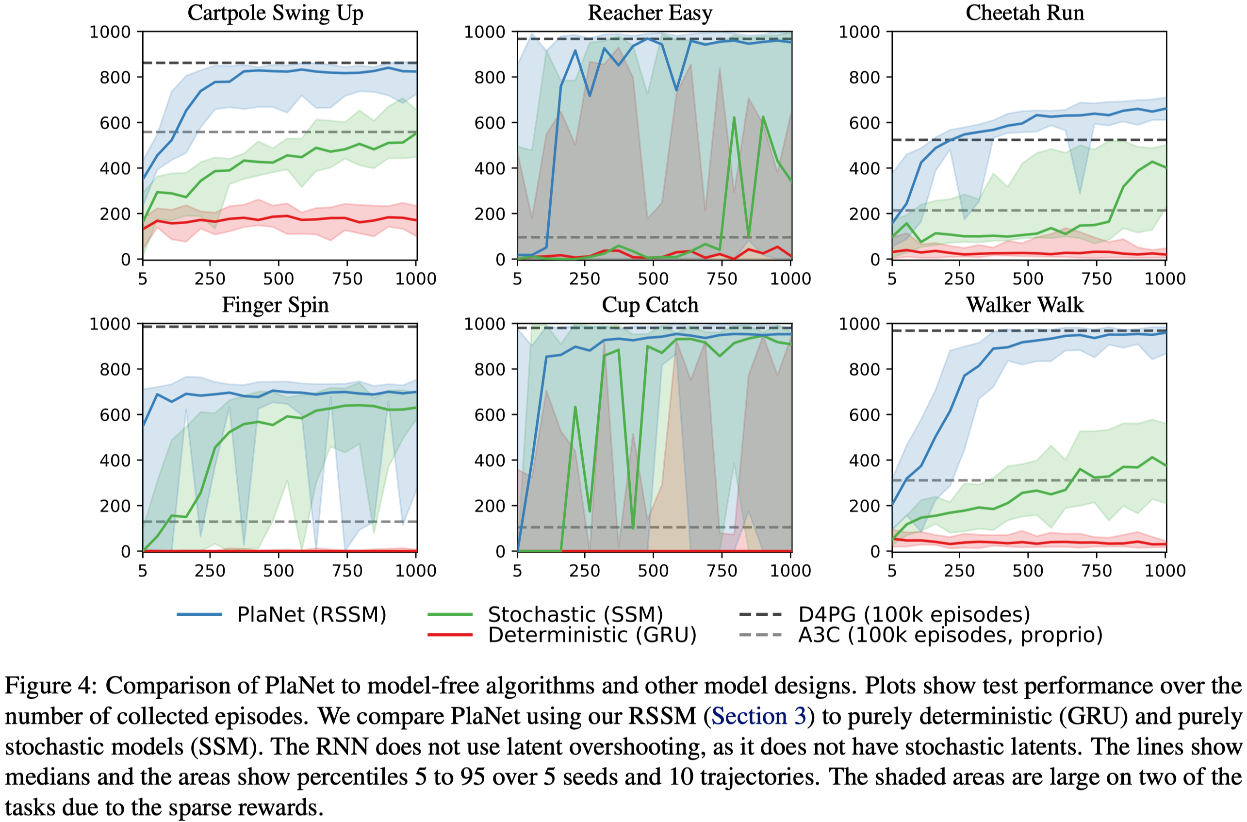
The deterministic and stochastic state models serve different purposes: The deterministic part enables the agent to reliably retain information across many time steps, while the stochastic part forms a compact belief state of the environment. The latter is especially important as the environment is generally partially observable to the agent – Figure 4 shows that, without the stochastic part, the agent fails to learn anything!
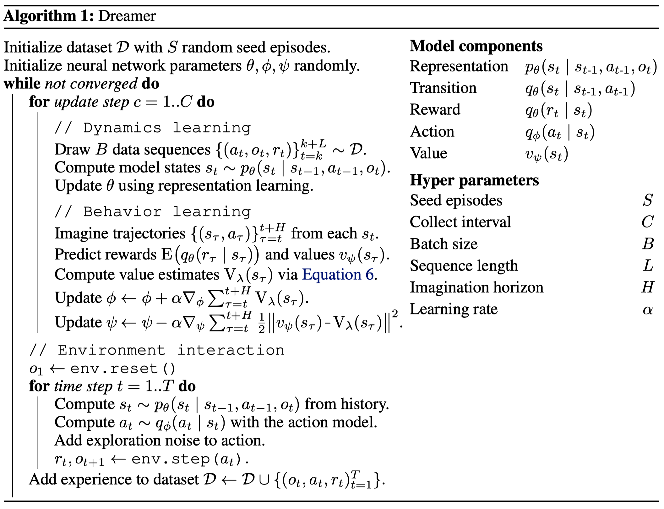
The input \(s_{t-1}\) to the deterministic model differs at the time of training the dynamics and actor-critic(AC) models. When training the dynamics, \(s_{t-1}\) comes from the posterior. When training the AC model, \(s_{t-1}\) is produced by the prior. These, as we’ll see soon, coincide with the corresponding loss functions. Figure 1 demonstrates this difference.

Reconstruction Loss

The dynamics model is trained with the reconstruction loss defined based on the following information bottleneck objective

\[\begin{align} \max \underbrace{I(s_{1:T};(o_{1:T},r_{1:T})|a_{1:T})}_{\text{MI in decoder}}-\beta \underbrace{I(s_{1:T}, o_{1:T}|a_{1:T})}_{\text{MI in encoder}}\tag {1} \end{align}\]

where \(\beta\) is a hyperparameter that controls the information penalty from \(o_{1:T}\) to \(s_{1:T}\). For ease of notation, \(s\) here stands for a state, which includes both \(s\) and \(h\) produced by the RSSM. Maximizing this objective leads to model states that predicts the sequence of observations and rewards while limiting the amount of information extracted at each time step. This encourages the model to reconstruct each image by relying on information extracted at preceding time steps to the extent possible, and only accessing additional information from the current image when necessary. As a result, the information regularizer encourages the model to learn long-term dependencies.

We can derive a lower bound on the generative objective using the non-negativity of the KL divergence and drop the marginal data probability that does not depend on the representation model

\[\begin{align} &I(s_{1:T};(o_{1:T},r_{1:T})|a_{1:T}))\\\ =&\mathbb E\big[\log p(o_{1:T},r_{1:T}|s_{1:T},a_{1:T})-\underbrace{\log p(o_{1:T},r_{1:T}|a_{1:T})}_{\text{independent of }s\text{, ignored}}\big]\\\ =&\mathbb E\left[\log p(o_{1:T}, r_{1:T}|s_{1:T},a_{1:T})\right]\\\ \ge&\mathbb E\left[\log p(o_{1:T}, r_{1:T}|s_{1:T},a_{1:T})\right]-D_{KL}[p(o_{1:T}, r_{1:T}|s_{1:T},a_{1:T})\Vert q(o_{1:T},r_{1:T}|s_{1:T})]\\\ =&\mathbb E\left[\log q(o_{1:T},r_{1:T}|s_{1:T})\right]\\\ =&\mathbb E\left[\sum_t\log q(o_t|s_t)+\log q(r_t|s_t)\right]\tag {2} \end{align}\]

Similarly, we can derive an upper bound for the second term

\[\begin{align} &I(s_{1:T};o_{1:T}|a_{1:T})\\\ =&\mathbb E\left[\sum_t\log p(s_t|s_{t-1},a_{t-1},o_t)-\log p(s_t|s_{t-1},a_{t-1})\right]\\\ \le&\mathbb E\left[\sum_t\log p(s_t|s_{t-1},a_{t-1},o_t)-\log p(s_t|s_{t-1},a_{t-1})\right]\\\ &\quad+D_{KL}\left[p(s_t|s_{t-1},a_{t-1})\Vert q(s_t|s_{t-1},a_{t-1})\right]\\\ =&\mathbb E\left[\sum_t\log p(s_t|s_{t-1},a_{t-1},o_t)-\log q(s_t|s_{t-1},a_{t-1})\right]\\\ =&\mathbb E\left[\sum_t D_{KL}\left[p(s_t|s_{t-1},a_{t-1},o_t)\Vert q(s_t|s_{t-1},a_{t-1})\right]\right]\tag {3} \end{align}\]

Together, Equations \((2)\) and \((3)\) give us the following lower bound of Equation \((1)\)

\[\begin{align} \mathbb E\left[\sum_t\log q(o_t|s_t)+\log q(r_t|s_t)-\beta D_{KL}\left[p(s_t|s_{t-1},a_{t-1},o_t)\Vert q(s_t|s_{t-1},a_{t-1})\right]\right]\tag {4} \end{align}\]

Acute readers may have noticed that Equation \((4)\) is, in fact, the variational evidence lower bound(ELBO) commonly seen in VAE. Indeed, we can regard the dynamics model as a sequential VAE, where the representation model is the encoder, the observation and reward models are the decoders, and the RSSM in between introduces sequential relations.

Behavior Learning

Dreamer learns an actor-critic(AC) architecture in the latent space, which makes it hard to use the real transitions to train the AC because the dynamics of latent space shifts as the dynamics model evolves. Therefore, Hafner et al. propose training the AC using imagined trajectories derived from the dynamics model(similar idea was first studied in Dyna). That is, the agent first imagine sequences starting from some true model states \(s_\tau\) from the agent’s past experience, following the transition model \(q(s_{t+1}\vert s_{t},a_{t})\), the reward model \(q(r_t\vert s_t)\), and policy \(q(a_t\vert s_t)\). Then it maximizes the exepcted imagined returns, which results in the following objective

\[\begin{align} \max_{\phi}\mathbb E_{q_\theta,q_\phi}&\left[\sum_{\tau=t}^{t+H}V_{\lambda}(s_\tau)\right]\\\ \min_{\psi}\mathbb E_{q_\theta,q_\phi}&\left[\sum_{\tau=t}^{t+H}{1\over 2}\Vert v_{\psi}(s_\tau)-V_\lambda(s_\tau)\Vert^2\right]\\\ where\quad V_\lambda(s_\tau)&=(1-\lambda)\sum_{n\ge 0}\lambda^{n}V^{n+1}(s_\tau)\\\ &=(1-\lambda)\sum_{n\ge 0}\lambda^{n}\left(\sum_{i=0}^{n}\gamma^ir_{\tau+i}+\gamma^{n+1}v_\psi(s_{t+n+1})\right)\\\ &=(1-\lambda)\sum_{i\ge 0}\gamma^ir_{\tau+i}\sum_{n\ge i}\lambda^{n}+(1-\lambda)\sum_{n\ge 0}\gamma^{n+1} v_\psi(s_{\tau+n+1})\\\ &=\sum_{n\ge 0}(\lambda\gamma)^nr_{\tau+n}+(1-\lambda)\gamma^{n+1} v_\psi(s_{\tau+n+1})\\\ &=r_\tau+(1-\lambda)\gamma v_\psi(s_{\tau+1})+\lambda\gamma\sum_{n\ge 0}(\lambda\gamma)^nr_{\tau+1+n}+(1-\lambda)\gamma^{n+1} v_\psi(s_{\tau+2+n})\\\ &= r_\tau+(1-\lambda)\gamma v_\psi(s_{\tau+1})+\lambda \gamma V_\lambda(s_{\tau+1}) \tag5 \end{align}\]

where \(\theta\) is the parameters of the dynamics model, and \(\phi,\psi\) are the parameters of action and value models, respectively. \(V_\lambda(s_t)\) is just the \(\lambda\)-return in TD(\(\lambda\)), where \(\lambda\) controls the bias and variance trade-off. Equation \((5)\) gives a recursive approach to compute the \(\lambda\)-return.

In fact, the choice of these RL objectives is quite brilliant. I’ve tried to apply some other off-policy methods to the latent space learned by Dreamer, such as SAC with retrace(\(\lambda\)), as I thought that function approximation errors introduced by the world model(i.e., the dynamics, reward, and discount models) might cause inaccurate predictions on the imagined trajectories, whereby impairing the performance of the AC model. However, the experimental results suggested an opposite story: learning from imagined trajectories outperforms applying off-policy methods on the latent space in terms of the learning speed and final performance. I hypothesize three reasons: 1. Learning from imagined trajectories provides richer training signals, facilitating the learning process. These can be seen from the observation that if we reduce the length of the imagined trajectories to \(1\), Dreamer performs worse than applying SAC to the latent space. 2. I only experiment on a small set of environments where Dreamer performs well. Specifically, for these environments, Dreamer can learn a reasonably well dynamics model, which inherently introduces some bias towards Dreamer. 3. Model-free algorithms rely on the assumption of a fixed dynamics, but the dynamics of the latent space constantly changes.

Pseudocode

References

Danijar Hafner, Timothy Lillicrap, Jimmy Ba, Mohammad Norouzi. Dream to Control: Learning Behaviors by Latent Imagination. In ICLR 2020

Alexander A. Alemi, Ian Fischer, Joshua V. Dillon, Kevin Murphy. Deep Variational Information Bottleneck. In ICLR 2017

Supplementary Materials

Reward prediction

The first approach is to predict future rewards from actions and past observations. This resembles the reward loss in MuZero, but it does not work well with Dreamer. As there is no official explanation for the poor performance, I personally conjecture three reasons:

MuZero uses more data throught the training process.
MuZero makes decision using MCTS, which gives training data of better quality.
MuZero learns the value and policy using the true experiences collected by the agent and propagates these gradients back through the representation model, while Dreamer learns these models from the imagined experiences and gradients.

Contrastive estimation

Image reconstruction requires high model capacity. We can derive a noise InfoNCE from Equation \((2)\) to avoid such overhead,

\[\begin{align} &\mathbb E\left[\log q(o_t|s_t)\right]\\\ =&\mathbb E\left[\log{q(o_t,s_t)\over q(s_t)}\right]\\\ =&\mathbb E\left[\log q(s_t|o_t) + \underbrace{\log q(o_t)}_{\text{independent of }s\text{, ignored}}-\log q(s_t)\right]\\\ =&\mathbb E\left[\log q(s_t|o_t) -\log q(s_t)\right]\\\ =&\mathbb E\left[\log q(s_t|o_t)-\log\sum_{o'}q(s_t|o')q(o')\right]\\\ \ge&\mathbb E\left[\log q(s_t|o_t)-\log \sum_{o'}q(s_t|o')\right]\tag {4} \end{align}\]

where the inequality holds because \(0<q(o’)\le1\).