
Introduction
We discuss DreamerV2, the successor of Dreamer that achieves high performance on Atari games comparable to state-of-the-art single-agent model-free algorithms.
DreamerV2
World Model Learning
World Model

DreamerV2 uses the same word model as Dreamer, comprised of an encoder for image embedding, an RSSM model for sequential modeling, and a set of decoders for predictions. We briefly summarize these model as follows
\[\begin{align} &\text{Recurrent model:}&h_t=f_\phi(h_{t-1},s_{t-1},a_{t-1})\\\ &\text{Representation model:}&s_t\sim q_\phi(s_t|h_t, x_t)\\\ &\text{Transition model:}&s_t\sim p_\phi(s_t|h_t)\\\ &\text{Observation predictor:}&x_t\sim p_\phi(x_t|h_t,s_t)\\\ &\text{Reward predictor:}&r_t\sim p_\phi(r_t|h_t,s_t)\\\ &\text{Discount predictor:}&\gamma\sim p_\phi(\gamma_t|h_t,s_t) \end{align}\tag 1\]The image predictor outputs the mean of a diagonal Gaussian likelihood with unit variance, the reward predictor outputs a univariate Gaussian with unit variance, and the discount predictor outputs a Bernoulli likelihood. The recurrent model is a Gated Recurrent Unit. The representation and transition models now produce a vector of several categorical variables as the stochastic state; For Atari games, there are \(32\) categorical variables, each of \(32\) dimensions. The representation and transition models are optimized using straight-through gradients, which are implemented as follows
def get_sample(logits):
  sample = one_hot(draw(logits))
  probs = softmax(logits)
  sample = sample + probs - stop_grad(probs)
  return sample
The reason why the categorical variables are beneficial is unclear, Hafner et al. 2020 hypothesize that
- A categorical prior can perfectly fit the aggregate posterior, because a mixture categorical is again a categorical. In contrast, a Gaussian prior cannot match a mixture of Gaussian posteriors, which could make it difficult to predict multi-modal changes between one image and the next.
- The level of sparsity enforced by a vector of categorical latent variables could be beneficial for generalization. Flattening the sample from the \(32 \) categorical variables with \(32\) classes each results in a sparse binary vector of length \(1024\) with \(32\) active bits.
- Despite common intuition, categorical variables may be easier to optimize than Gaussian variables, possibly because the straight-through gradient estimator ignores the reparameterization that would otherwise scale the gradient. This could reduce exploding and vanishing gradients.
- Categorical variables could be a better inductive bias than unimodal continuous latent variables for modeling the non-smooth aspects of Atari games, such as when entering a new room, or when collected items or defeated enemies disappear from the image.
World Model Loss
The world model loss is a variant of the ELBO objective defined by
\[\begin{align} \mathcal L=\mathbb E\Big[\sum_t&\underbrace{-\eta_x\log p_\phi(x_t|h_t, s_t)}_\text{image loss}\underbrace{-\eta_r\log p_\phi(r_t|h_t, s_t)}_\text{reward loss}\underbrace{-\eta_\gamma\log p_\phi(\gamma_t|h_t,s_t)}_\text{discount loss} \\\ &\underbrace{-\eta_t\log p_\phi(s_t|h_t)}_\text{transition loss}+\underbrace{\eta_q\log q_\phi(s_t|h_t,x_t)}_\text{latent entopy regularizer}\Big]\\\ where\quad(\eta_x,\eta_r,\eta_\gamma,\eta_t,\eta_q)&=(1/(64\cdot64\cdot3), 1, 1, 0.08, 0.02) \end{align}\]where the first three terms are reconstruction loss and the latter two together are the KL divergence between the representation and transition model. We here split the KL divergence into two terms so that we can use different coefficients. Hafner et al. 2020 refer to this as KL balancing. It allows us to reduce the KL by encouraging learning an accurate transition function instead of increasing posterior entropy.
Behavior Learning
Critic Loss
For critic loss, DreamerV2 uses TD(\(\lambda\)) loss as Dreamer:
\[\begin{align} \mathcal L(\psi)=&\mathbb E_{\pi_\theta,p_\phi}\left[{1\over H-1}\sum_{t=1}^{H-1}{1\over 2}\Vert v_{\psi}(s_t)-V_\lambda(s_t)\Vert^2\right]\\\ where\quad V_\lambda(s_t)=&r_t+\gamma\begin{cases} (1-\lambda)v_{\bar\psi}(s_{t+1})+\lambda V_\lambda(s_{t+1})& \text{if }\tau < H\\\ v_{\bar\psi}(s_{H})&\text{if }\tau=H \end{cases} \end{align}\]Different from Dreamer, the target value is computed using a target network that is updated every \(100\) gradient steps.
Actor Loss
Dreamer computes gradient by directly maximizing the \(\lambda\)-return. This is biased as \(v_\psi\) is inaccurate. Therefore, DreamerV2 further introduces the high-variance Reinforce gradients. The final actor loss is
\[\begin{align} \mathcal L(\theta)=\mathbb E_{\pi_\theta,p_\phi}\Big[{1\over H-1}\sum_{t=1}^{H-1}\big(\underbrace{-\eta_s \log \pi_\theta(a|s)(V_\lambda(s_t)-v_\psi(s_t))}_\text{reinforce}\underbrace{-\eta_dV_\lambda(s_t)}_\text{dynamic backprop}\ \underbrace{-\eta_e\mathcal H(\pi_\theta)}_\text{entropy regularizer}\big)\Big] \end{align}\]where \(\eta_s=0.9\) and, over the first 10M environment frames, \(\eta_d=0.1\rightarrow 0\) and \(\eta_e=3\times 10^{-3}\rightarrow3\times 10^{-4}\). Experiments show that policy gradient contributes most to the success of DreamerV2.
When explaining the efficacy of Reinforce gradients, Hafner et al. 2021 ascribe it to the unbiasedness of Reinforce gradient. However, this is not true as \(V_\lambda\) is biased.
I personally conjecture a reason why maximizing TD(\(\lambda\)) performs worse than Reinforce. When maximizing TD(\(\lambda\)), the gradients were first flowed through the world model \(p(s’\vert s,a)\) then the policy model. This could possibly causes two problems: 1) the error of the world model may be propagated to the policy model, resulting in inaccurate gradient estimates. 2) the vanishing/exploding gradient problem may occur as now the prediction graph becomes very deep and there is no mechanism such as skip connection to deal with the problem—though this problem might be partially addressed by the intermediate policy losses at each imagine step.
Summary of Modification
We list a summary of changes that were tried and were found to helpful:
- Categorical latents. Using categorical latent states and straight-through gradients in the world model instead of Gaussian latents with reparameterized gradients.
- Mixed actor gradients. Combining Reinforce and dynamics backpropagation gradients for learning the actor instead of dynamics backpropagation only.
- Policy entropy. Regularizing the policy entropy for exploration both in imagination and during data collection, instead of using external action noise during data collection.
- KL balancing. Separately scaling the prior cross entropy and the posterior entropy in the KL loss to encourage learning an accurate temporal prior, instead of using free nats.
- Model size. Increasing the number of units or feature maps per layer of all model components, resulting in a change from 13M parameters to 22M parameters.
- Layer norm. Using layer normalization in the GRU that is used as part of the RSSM latent transition model, instead of no normalization.
Summary of changes that were tried but were not shown to help:
-
Binary latents. Using a larger number of binary latents for the world model instead of using categorical latents, which could have encouraged a more disentangled representation.
-
Long-term entropy. Including the policy entropy into temporal-difference loss of the value function, so that the actor seeks out states with high action entropy beyond the planning horizon.
-
Scheduling. Scheduling the learning rate, KL scale, free bits. Only scheduling the entropy regularizer and the amount of straight-through gradients for the policy was beneficial.
-
Reinforce only. Using only Reinforce gradients for the actor worked for most games but led to lower performance on some games, possibly because of the high variance of Reinforce gradients.
Experimental Results
We don’t discuss the comparison between DreamerV2 and DQN families as the comparison is not fair. On one hand, DreamerV2 uses significantly more parameters(also a different architecture) than the model-free baselines used in comparison, which may help explain part of its superior performance. On the other hand, DreamerV2 takes smaller images as input than standard DQN families, which may cause some performance loss.
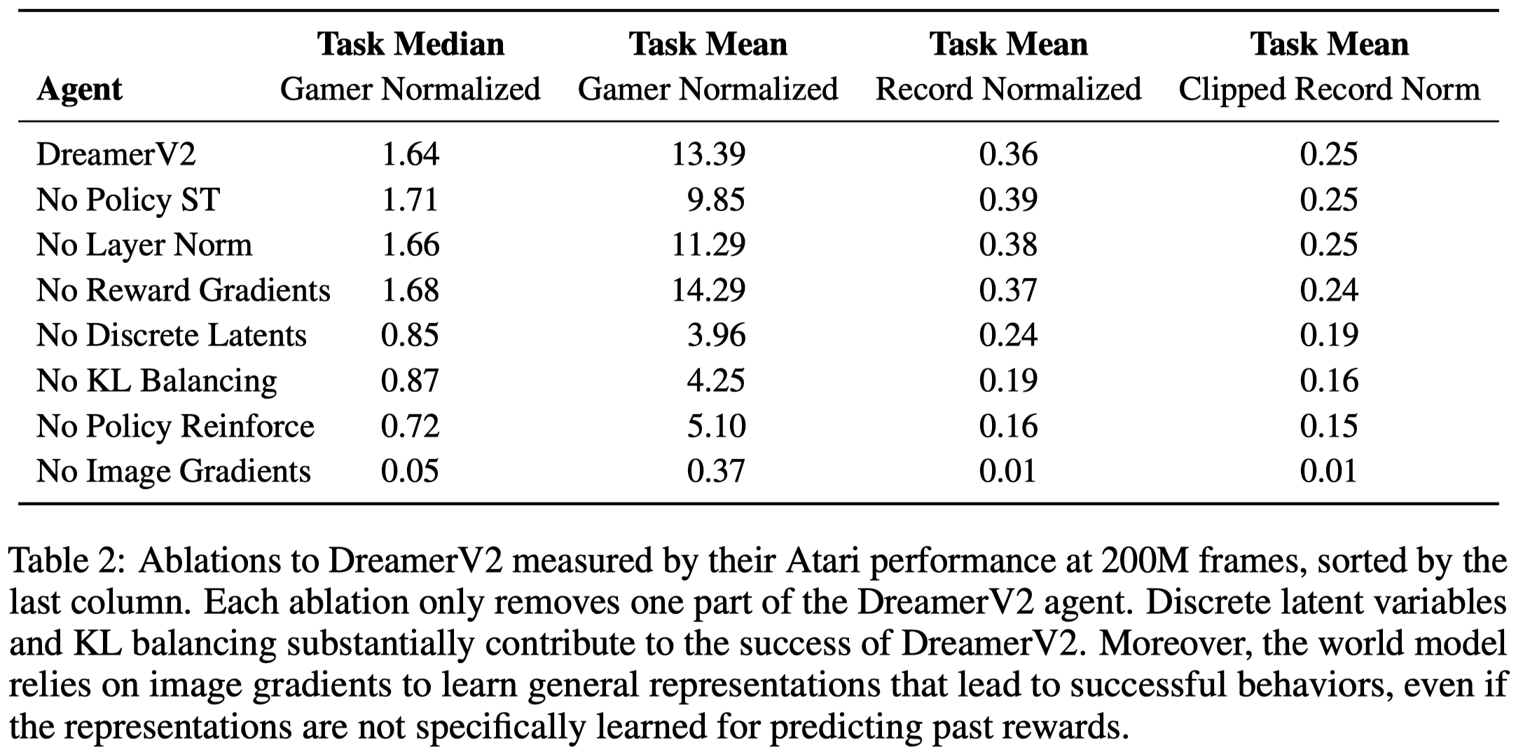
We summarize the ablation study on Atari below
- Categorical latents. Categorical latent variable outperform than Gaussian latent variables on \(42\) tasks, achieve lower performance on \(8\) tasks, and are tied on \(5\) tasks
- KL balancing. KL balancing outperforms the standard KL regularizer on \(44\) tasks, achieves lower performance on \(6\) tasks, and is tied on \(5\) tasks.
- Model gradients. Stopping the image gradients increases performance on \(3\) tasks, decreases performance on \(51\) tasks, and is tied on \(1\) task. Thus, the world model of DreamerV2 thus heavily relies on the learning signal provided by the high-dimensional images. Stopping the reward gradients increases performance on \(15\) tasks, decreases performance on \(22\) tasks, and is tied on \(18\) tasks. The difference of using reward gradients is small.
- Policy gradients. Using only Reinforce gradients to optimize the policy increases performance on \(18\) tasks, decreases performance on \(24\) tasks, and is tied on \(13\) tasks. Table 2 shows that it even results in better task median(No Policy ST); mixing Reinforce and straight-through gradients yields a substantial improvement on James Bond and Seaquest, leading to a higher gamer normalized task mean scores. Using only straight-through gradients to optimize the policy increases performance on \(5\) tasks, decrease performance on \(44\) tasks, and is tied on \(6\) tasks.
References
Hafner, Danijar, Timothy Lillicrap, Mohammad Norouzi, and Jimmy Ba. 2020. “Mastering Atari with Discrete World Models.” ArXiv, 1–24.