
Introduction
GAIL, proposed by Ho et al. 2016, has been one of the most widely used imitation learning algorithms since it was published. In this post, we present a concise theoretical analysis on it.
Note. Different from the paper, we in this post describe GAIL in the reward maximization paradigm rather than the cost minimization framework.
Preliminaries
MaxEnt IRL
In MaxEnt IRL, we define the following optimization problem
\[\begin{align} \min_r\max_\pi\mathbb E_\pi[r(s,a)]+\mathcal H(\pi)-\mathbb E_{\pi_E}[r(s,a)]\tag 1 \end{align}\]where \(\mathbb E_\pi[r]\) and \(\mathcal H(\pi)\) are \(\gamma\)-discounted trajectory rewards and entropy, respectively, and we omit domains whenever it does not cause any ambiguity.
Because IRL learned from a finite expert dataset can easily overfit, we introduce a convex regularizer: \(\psi:\mathbb R^{\mathcal S\times\mathcal A}\rightarrow \mathbb R\)—the regularizer is assumed to be convex because we want to learn a reward function that minimizes it. Now we define the regularized IRL objective
\[\begin{align} \text{IRL}_\psi(\pi_E)=\arg\min_r\psi(r)+(\max_\pi\mathbb E_\pi[r(s,a)]+\mathcal H(\pi))-\mathbb E_{\pi_E}[r(s,a)]\tag 2 \end{align}\]Occupancy measure
For a policy \(\pi\in \Pi\), define its occupancy measure \(\rho_\pi:\mathcal S\times\mathcal A\rightarrow \mathbb R\) as \(\rho_\pi(s,a)=\pi(a\vert s)\sum_{t=0}^\infty\gamma^t P(s_t=s\vert \pi)\), which is the \(\gamma\)-discounted state-action visitation distribution of policy \(\pi\). It allows us to write \(\mathbb E_\pi[r(s,a)]=\sum_{s,a}\rho_\pi(s,a)r(s,a)\) for any reward function \(r\). Define the set of valid occupancy measures \(\mathcal D={\rho_\pi:\pi\in\Pi}\). It’s easy to see that there is a one-to-one correspondence between \(\Pi\) and \(\mathcal D\). Furthermore, we have
-
\(\pi_\rho=\rho(s,a)/\sum_{a’}\rho(s,a’)\).
-
\(\rho(s,a)=\pi_\rho(a\vert s)\rho(s)\), where \(\rho(s)\) is the discounted state visitation distribution.
-
\(\mathcal H(\pi)=\bar{\mathcal H}(\rho_\pi)\) and \(\bar{\mathcal H}(\rho)=\mathcal H(\pi_\rho)\), where \(\bar{\mathcal H}(\rho)=-\sum_{s,a}\rho(s,a)\log\pi_\rho(s,a)\) and \(\mathcal H(\pi)=-\sum_s\rho_\pi(s)\sum_a\pi(a\vert s)\log\pi(s,a)\)
-
an equivalent of Equation \((2)\):
Characterizing the induced optimal policy
Let \(\text{RL}(r)\) be the policy learned by RL with the reward function \(r\) and \(\text{IRL}(\pi_E)\) be the reward function recovered by IRL from the expert policy \(\pi_E\).
Proposition 3.2 \(\text{RL}\circ\text{IRL}(\pi_E)=\arg\max_{\pi}\mathcal H(\pi)-\psi^*(\rho_{\pi_E}-\rho_\pi)\).
The proof is given in Appendix, but it’s worth stressing that \(\pi\) and \(\rho_\pi\) are interchangeable.
Proposition 3.2 tells us that \(\psi\)-regularized IRL implicitly seeks a policy whose occupancy measure is close to the expert’s. Enticingly, this suggests that various settings of \(\psi\) lead to various imitation learning algorithms that directly solve the optimization problem given by Proposition 3.2.
Corollary 3.2.1 If \(\psi\) is a constant function, \(\tilde r\in\text{IRL}(\pi_E)\), and \(\tilde \pi\in\text{RL}(\tilde r)\), then \(\rho_{\tilde \pi}=\rho_{\pi_E}\).
Proof. Let \(\bar{\mathcal L}(\rho_\pi,r)=\bar {\mathcal H}(\rho_\pi)-\sum_{s,a}(\rho_{\pi_E}(s,a)-\rho_{\pi}(s,a))r(s,a)\). We can see that \(\tilde r\in\arg\min_r\max_{\rho_\pi}\bar{\mathcal L}(\rho_\pi,r)\) is the dual of the following optimization problem
\[\begin{align} \max_{\rho_\pi}\bar{\mathcal H}&(\rho_\pi)\tag 3\\\ s.t.\quad \rho_\pi(s,a)=&\rho_{\pi_E}(s,a)\quad\forall s\in\mathcal S,a\in\mathcal A \end{align}\]with \(\tilde r\) being the dual optimum. Because of the strict concavity of \(\bar{\mathcal H}\), the primal optimum is obtained when the constraint is satisfied, i.e., \(\rho_{\tilde \pi}=\rho_{\pi_E}\)
From Corollary 3.2.1, we deduce that
- IRL is a dual of an occupancy measure matching problem, and the recovered reward function is the dual optimum.
- The induced optimal policy is the primal optimum.
Method
Corollary 3.2.1 is not useful in practice as, in reality, the expert trajectory distribution is unknown and instead is often provided as a finite set of samples. Therefore, we relax Equation \((3)\) into the following form, motivated by Proposition 3.2
\[\begin{align} \max_\pi \mathcal H(\pi)-\psi^\*(\rho_{\pi_E}-\rho_\pi)\tag 4 \end{align}\]Ho et al. 2016 propose the following conjugate
\[\begin{align} \psi^\*_{GA}(\rho_{\pi_E}-\rho_\pi)=\max_{D}\mathbb E_\pi[\log(1-D(s,a))]+\mathbb E_{\pi_E}[\log(D(s,a))]\tag 5 \end{align}\]which is exactly the discriminator objective in GANs. As in GANs, we can show that the optimal discriminator is \(D_*(s,a)={\pi_E(s,a)\over \pi_E(s,a)+\pi(s,a)}\) by taking the derivative of the above objective and setting it to zero. Furthermore, at the optimal point, this loss corresponds to the Jensen-Shannon divergence between policies up to a constant
\[\begin{align} \psi^\*_{GA}(\rho_{\pi_E}-\rho_\pi)=&\mathbb E_\pi\left[\log{\pi(s,a)\over\pi(s,a)+\pi_E(s,a)}\right]+\mathbb E_{\pi_E}\left[\log{\pi_E\over\pi(s,a)+\pi_E(s,a)}\right]\\\ =&\mathbb E_\pi\left[\log{\pi(s,a)\over{1\over 2}(\pi(s,a)+\pi_E(s,a))}\right]+\mathbb E_{\pi_E}\left[\log{\pi_E\over{1\over 2}(\pi(s,a)+\pi_E(s,a))}\right]-2\log 2\\\ =&2JSD(\pi\Vert\pi_E)-2\log 2 \end{align}\]\(\psi\) is convex
Remember that we claim that \(\psi\) should be a convex regularizer. Now we prove that the \(\psi_{GA}\) associated to \(\psi_{GA}^*\) is convex.
We start from the definition of \(\psi_{GA}^*\)
\[\begin{align} \psi_{GA}^\*(\rho_{\pi_E}-\rho_\pi)=&\sum_{s,a}\max_{D}\rho_\pi(s,a)\log(1-D(s,a))+\rho_{\pi_E}\log D(s,a)\\\ &\qquad\color{red}{D(s,a)={1\over1+e^{-f(s,a)}}\text{. From now on, we omit all }(s,a)\text{ for simplicity}}\\\ =&\sum_{s,a}\max_f\rho_\pi\log{1\over 1+e^{f}}+\rho_{\pi_E}\log{1\over 1+e^{-f}}\\\ &\qquad\color{red}{\phi(f)=\log{1+e^{f}}}\\\ =&\sum_{s,a}\max_f-\rho_\pi\phi(f)-\rho_{\pi_E}\phi(-f)\\\ =&\sum_{s,a}\max_f-\rho_\pi\phi(f)-\rho_{\pi_E}\phi(-\phi^{-1}(\phi(f)))\\\ &\qquad\color{red}{r=\phi(f)}\\\ =&\sum_{s,a}\max_r-\rho_\pi r-\rho_{\pi_E}\phi(-\phi^{-1}(r))\\\ =&\sum_{s,a}\max_r(\rho_{\pi_E}-\rho_{\pi})r -\rho_{\pi_E}(r-\phi(-\phi^{-1}(r)))\\\ \end{align}\]from which we deduce
\[\begin{align} \psi(r)=\begin{cases} \rho_{\pi_E}g(r)&{\text{if }r>0}\\\ \infty&\text{otherwise} \end{cases} \qquad g(r)=\begin{cases} r-\phi(-\phi^{-1}(r))&{\text{if }r>0}\\\ \infty&\text{otherwise} \end{cases} \end{align}\]Here, the condition is introduced because \(1-D={1\over\exp(\phi(f))}\in(0,1)\Rightarrow \exp(\phi(f))>1\Rightarrow r=\phi(f)> 0\).
Because \(\phi\) is concave and \(\phi^{-1}\) is convex, we have
\[\begin{align} \phi (-\phi^{-1}(tx+(1-t)y))\ge&\phi(-t\phi^{-1}(x)-(1-t)\phi^{-1}(y))\\\ \ge&t\phi(-\phi^{-1}(x))+(1-t)\phi(-\phi^{-1}(y)) \end{align}\]Therefore, \(\phi(-\phi^{-1}(r))\) is concave, inducing the convexity of \(g(r)\) and \(\psi(r)\).
Objectives
Sticking Equation \((5)\) into Equation \((4)\), we can see that GAIL essentially optimizes the following objectives
\[\begin{align} \min_D\mathcal L(D)=&-\mathbb E_\pi[\log(1-D(s,a))]+\mathbb E_{\pi_E}[\log D(s,a)]\\\ \max_\pi\mathcal J(\pi)=&\mathcal H(\pi)+\mathbb E_\pi[-\log(1-D(s,a))] \end{align}\]Experimental Results
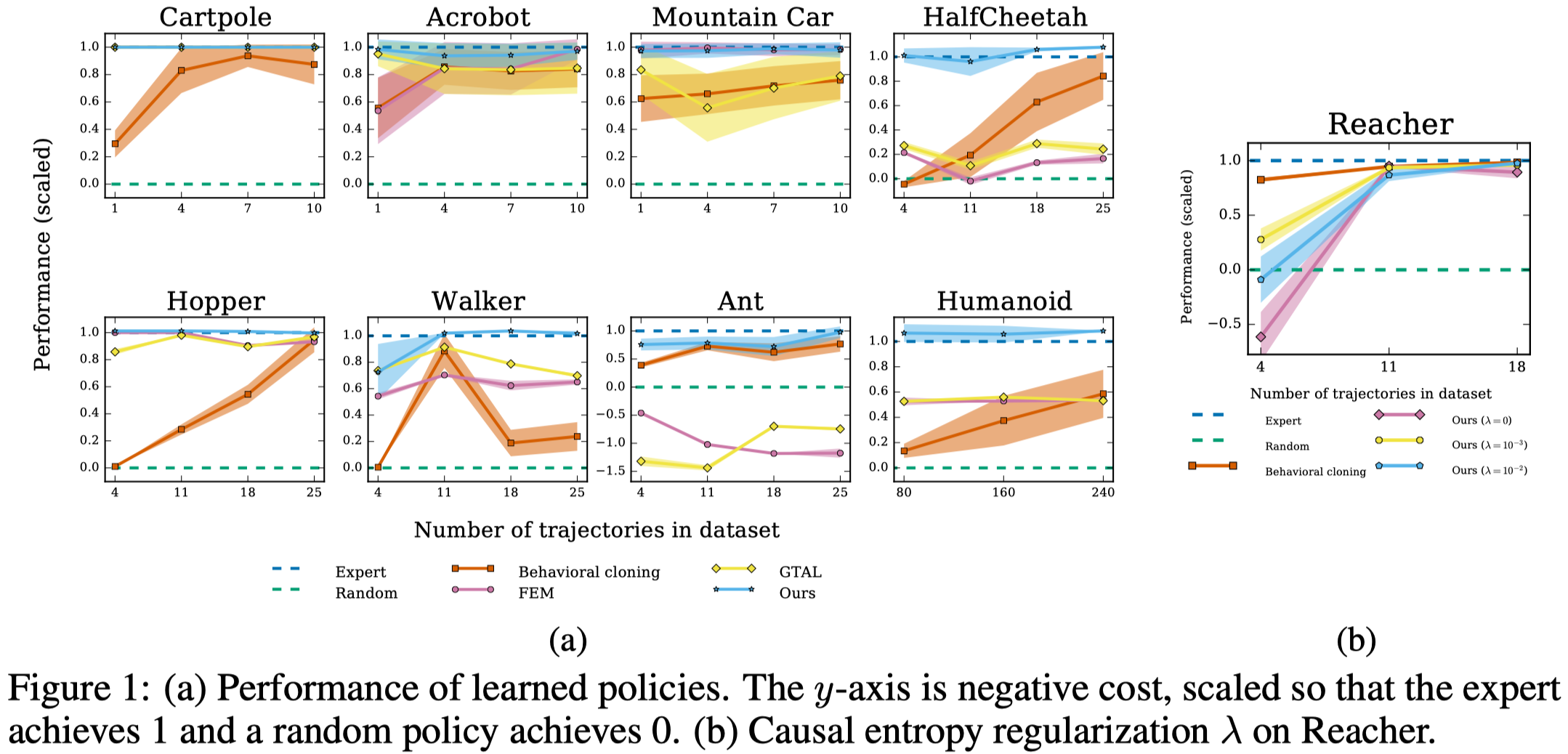
Figure 1 shows that GAIL performs extremely well across all tasks; it basically replicates the behavior of the expert data in all environments. Moreover, GAIL only requires a small number of expert trajectories.
References
Ho, Jonathan, and Stefano Ermon. 2016. “Generative Adversarial Imitation Learning.” Advances in Neural Information Processing Systems, 4572–80.
Appendix
Proofs
Proposition 3.2 \(\text{RL}\circ\text{IRL}(\pi_E)=\arg\max_{\pi}\mathcal H(\pi)-\psi^*(\rho_\pi-\rho_E)\).
Let \(\tilde r\in\text{IRL}(\pi_E)\) and \(\tilde \pi\in\text{RL}(\tilde r)=\text{RL}\circ\text{IRL}(\pi_E)\), and
\[\begin{align} \pi_A\in&\arg\max_\pi\mathcal H(\pi)-\psi^\*(\rho_{\pi_E}-\rho_{\pi})\\\ =&\arg\max_\pi\min_r\mathcal H(\pi)+\psi(r)-\sum_{s,a}(\rho_{\pi_E}(s,a)-\rho_{\pi}(s,a))r(s,a) \end{align}\]Let \(\rho_A\) be the occupancy measure of \(\pi_A\), \(\tilde \rho\) be the occupancy measure of \(\tilde \pi\), and define the Lagrangian
\[\begin{align} \bar{\mathcal L}(\rho_\pi,r)=\bar {\mathcal H}(\rho_\pi)+\psi(r)-\sum_{s,a}(\rho_{\pi_E}(s,a)-\rho_{\pi}(s,a))r(s,a) \end{align}\]Because of the one-to-one correspondence between a policy and its occupancy measure, we have
\[\begin{align} \rho_A\in\arg\max_{\rho_\pi}\min_r\bar{\mathcal L}(\rho_\pi,r) \end{align}\]By Equation \((3)\), we have
\[\begin{align} \tilde r\in&\arg\min_r\max_{\rho_\pi}\bar{\mathcal L}(\rho_\pi,r)\\\ \tilde \rho\in&\arg\max_{\rho_\pi}\bar{\mathcal L}(\rho_\pi,\tilde r) \end{align}\]Now we show \(\rho_A=\tilde \rho\). Because \(\mathcal H\) is concave and \(\psi\) is convex, we have that \(\bar{\mathcal L}(\cdot,r)\) is concave and \(\bar{\mathcal L}(\rho,\cdot)\) is convex. Therefore, by the minimax theorem, we have
\[\begin{align} \min_r\max_{\rho_\pi}\bar{\mathcal L}(\rho_\pi,r)=\max_{\rho_\pi}\min_r\bar{\mathcal L}(\rho_\pi,r) \end{align}\]This implies \(\rho_A=\tilde \rho\) and thus \(\pi_A=\tilde \pi\).