
Introduction
We discuss Go-Explore proposed by Ecoffet et al. 2021 on Nature. Go-Explore outperforms humans on all Atari57, and achieves incredibly good performance on hard-exploration games, such as Montezuma’s Revenge.
Despite its appealing results, there are three concerns needed to be aware of:
- Go-Explore requires the environment to be resettable to some specific state. Ecoffet et al. 2021 also propose training a goal-directed policy to circumvent this issue, which also outperforms SOTA algorithms and human performance in Montezuma’s Revenge and Pitfall. However, regarding the limited environments they test in, it’s still unclear if this is a general solution. Moreover, the robustification phase also requires resetting the environment.
- In the exploration phase, Go-Explore is only able to find the optimal open-loop trajectories. In other words, There is no learning happening here and subsequently there is no way to replicate these trajectories if the environment is stochastic. Learning actually happens in the robustification phase, where Go-Explore adopts the backward algorithm to learn from these optimal trajectories. However, the backward algorithm is extremely expensive. The good news is that the policy learned in the robustification phase is able to achieve performance comparable to, sometimes exceeding the one from the exploration phase.
- Due to the random exploration nature in the exploration phase, Go-Explore is sample inefficient(usually trained in the scale of billions of frames) on environments with dense rewards, compared to the contemporary SOTA algorithms such as Agent57.
Issues of Intrinsic-Motivated Exploration
The ineffectiveness of intrinsic-motivated exploration methods stems from two root causes that the authors call detachment and derailment:
-
Detachment describes that an agent driven by intrinsic reward could become detached from the frontiers of high intrinsic reward.
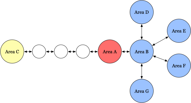
For example, as shown in the above figure, area A is connected to areas B and C. Without loss of generality, we assume C is a little farther from A and A and C is connected through a rewardless hallway and B contains some positive extrinsic reward that tempts the agent in the first place. The agent starts by exploring A, and after exhausting all the intrinsic reward offered by A, it turns to B. Provided that B is connected to some other area, after the agent has fully explored B, the agent then turns to another area connected to B and so on. It may be difficult for the agent to rediscover A and find a path to C, because it has already consumed the intrinsic reward in A, and it likely will not remember how to return to A due to catastrophic forgetting. This could be remedied by random initialization, replay buffers, and adding intrinsic rewards back over time. However, these strategies may not always be desirable: 1.) random initialization is in general not achievable for real-world problems; even in simulations, we always restrict initialization to small state space. 2.) replay buffers could prevent detachment in theory, but in practice, it would have to be large to prevent data about the abandoned frontier(A in the above example) from being purged before it becomes needed, and large replay buffers introduce their own optimization stability difficulties. 3.) Slowly adding intrinsic rewards back over time may not work as it indefinitely repeats the entire fruitless process.
-
Derailment describes that the agent cannot return to the state that is considered promising. Notice that we generally have two levels of exploration mechanisms in intrinsic-motivated agents: 1.) the intrinsic reward incentive that rewards when new states are reached, and 2.) the basic exploratory mechanism such as a stochastic policy. Importantly, intrinsic-motivated agents rely on the latter mechanism to discover states containing high intrinsic reward, and the former to return to them. However, the longer, more complex, and more precise a sequence of actions needs to be in order to reach a previously-discovered high-intrinsic-reward state, the more likely it is that exploration mechanisms(especially the basic exploration strategy) will “derail” the agent from ever returning to that state.
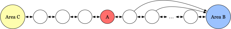
An extreme example is shown in the above figure. We assume A is a state, and leave B and C as areas. As before, we assume the agent is tempted to B in the first place. After it has fully explored B, it figured it might be a good idea to return A and try the left path. But the road back requires a long sequence of precise actions, which is hard to achieve because of the stochasticity introduced by the exploration mechanisms.
Go-Explore avoids these problems by storing an archive of promising states so that the agent can return to them later (i.e., resetting the simulator to that state).
Go-Explore
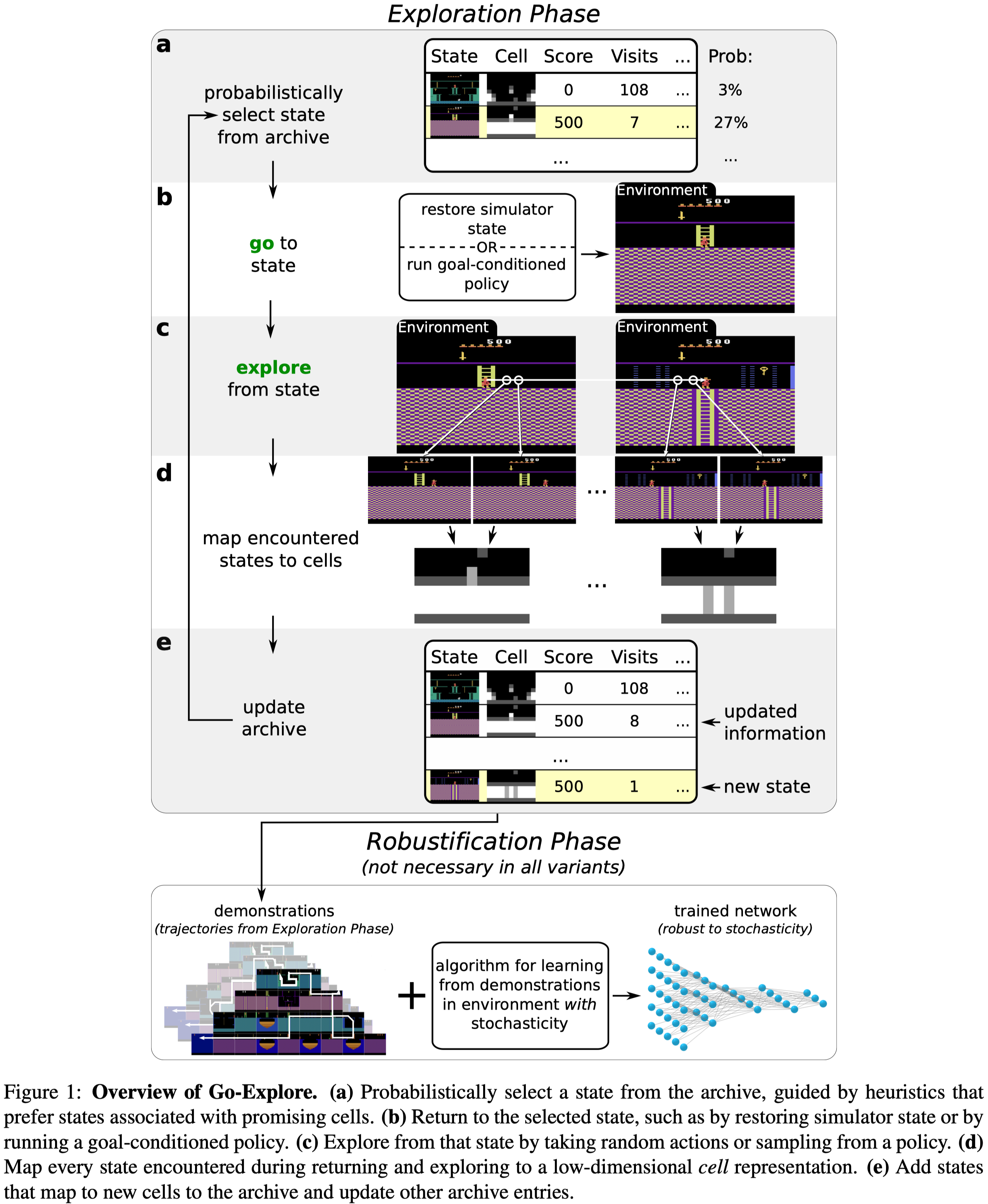
Go-Explore consists of two phases: In Phase 1, it maintains an archive that records promising(novel) states. At each iteration, the agent first returns to one of the states in the archive, and then takes actions to explore the environment for \(k\) steps, adding novel states and associated trajectories to the archive. In Phase 2, it learns a policy through the backward algorithm.
Note that 1) Phase 1 may not involve any network training if random actions are used for exploration; 2) Due to the prohibitive cost of the backward algorithm, the robustification phase may be omitted if we only need good trajectories for the game, in which case, no learning is performed.
Select State from The Archive
Cells are selected inversely proportional to its visited count with weight \(W={1\over\sqrt {C_{seen}}+1}\), where \(C_{seen}\) is the number of times the cell is revisited.
Go to state
Go-Explore assumes the environment is deterministic during training and stochastic in test time. A deterministic environment ensures that we can always return to states that we found promising by following the sequence of actions taken before. Furthermore, we might store the state of the simulator and restore it later.
Ecoffet et al. 2021 also propose a policy-based version to return to the selected state and relax the deterministic and resettable requirements for the environment. The agent’s policy is implemented as a goal-conditioned PPO, where the goal is a concatenated one-hot encoding of the cell. Because it is hard for a policy to learn from a distant goal, we select a sequence of goals from the trajectory associated to the selected state. Whenever the agent meets a goal, it receives 1 reward and selects a subsequent goal to condition on. We refer readers to Page20 of Ecoffet et al. 2021 for more details.
Exploration
Go-Explore explores by taking random actions for \(k=100\) training frames, with a \(95\%\) probability of repeating the previous action at each training frame.
Cell Representations
In Go-Explore, Ecoffet et al. 2021 adopt an engineering method for downsampling, which consists of three steps
- Convert the original frame to grayscale
- Reduce the resolution with pixel area relation interpolation to a width \(w\le 160\) and a height \(h\le 210\)
- Reduce the pixel depth to \(d\le 255\) using the formula \(\lfloor {d\cdot p\over 255}\rfloor\), where \(p\) is the value of the pixel after step \(2\).
The parameters \(w, h, d\) are updated dynamically by proposing different values for each, calculating how a sample of recent frames would be grouped into cells under these proposed parameters, and then selecting the values that result in the best cell distribution (as determined by the objective function below)
Let \(n\) be the number of cells produced by the parameters currently considered, \(T\) be a target number of cells(a fixed fraction(\(12.5\%\)) of the number of frames(code) in the sample), \(\pmb p\) be the distribution of sample frames over cells. The objective function for candidate downscaling parameters is calculated by
\[\begin{align} O(\pmb p,n)=&{H_n(\pmb p)\over L(n,T)}\\\ where\quad H_n(\pmb p)=&{-\sum_i p_i\log p_i\over\log n}\\\ L(n,T)=&\sqrt{\left\vert{n\over T}-1\right\vert+1} \end{align}\]Here \(H_n(\pmb p)\) is the normalized entropy, which preserves the scale of the entropy regardless of \(n\). This term encourages frames to be distributed as uniformly as possible across cells. \(L(n,T)\) measures the discrepancy between the number of cells produced by the current parameters and the target number of cells. It prevents from aggregating frames into too many or too few cells.
At each step of the randomized search, new values of each parameter \(w,h,d\) are proposed by sampling from a geometric distribution whose mean is the current best-known value of the given parameter. If the current best-known value is lower than a heuristic minimum mean, the heuristic mean is used instead. New parameter values are re-sampled if they fall outside of the valid range of the parameter.
The recent frames that constitute the sample over which parameter search is done are obtained by maintaining a set of recently seen sample frames as Go-Explore runs: during the exploration phase, a frame not already is added to the running set with a probability of \(1\%\). If the resulting set contains more than 10,000 frames, the oldest frame it contains is removed.
We omit the domain knowledge representations and refer interested readers to the paper.
Update Archive
Cells and the corresponding state and trajectories are added to the archive if it does not yet exist in the archive. For cells already in the archive, if it’s associated with a better trajectory (e.g., higher performance or shorter), that state and its associated trajectory will replace the state and trajectory current associated with that cell.
Robustification
It works by starting the agent near the last state in the trajectory and then running an ordinary RL algorithm from there (in this case, PPO+SIL). Once the algorithm has learned to obtain the same or a higher reward than the example trajectory from that starting place near the end of the trajectory, the algorithm backs the agent’s starting point up to a slightly earlier place along the trajectory and repeats the process until eventually, the agent has learned to obtain a score greater than or equal to the example trajectory all the way from the initial state.
Self-Imitation Learning
Besides PPO, a small number of workers are devoted to self-imitation learning(SIL). Instead of running the learned policy, these workers replay trajectories associated to the selected cells. The replayed data is then used to update the SIL loss
\[\begin{align} \mathcal L^{SIL}=&\mathcal L^{SIL\_PG}+w_{SIL\_VF}\mathcal L^{SIL\_VF}+w_{SIL\_ENT}\mathcal L^{SIL\_ENT}\\\ \mathcal L^{SIL\_PG}=&\mathbb E[-\log\pi(a|s)\max(0, R-V(s))]\\\ \mathcal L^{SIL\_VF}=&\mathbb E[{1\over 2}\max(0,R-V(s))^2] \end{align}\]where \(R\) is the discounted trajectory return.
Experimental Results
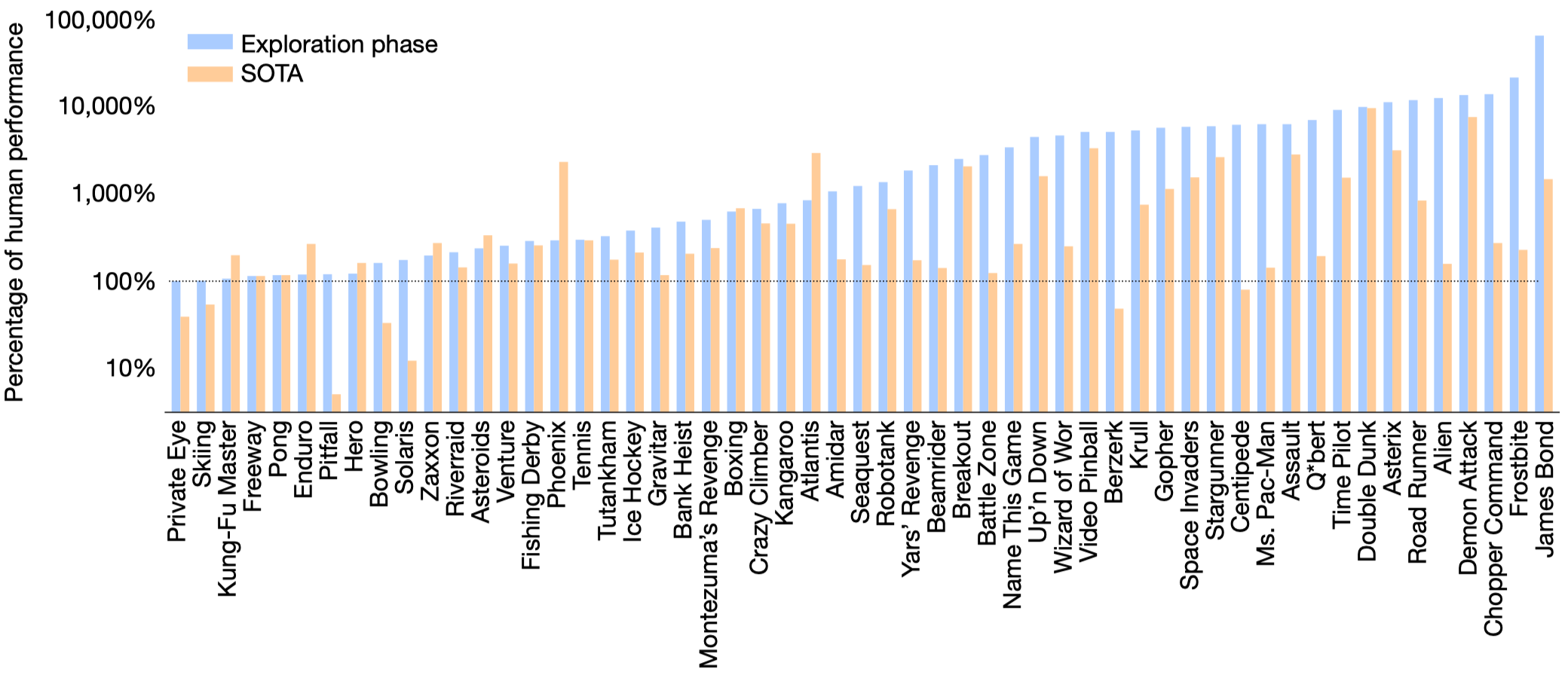
Figure 3 shows promising results of Go-Explore. However, the SOTA excludes Agent57 as the latter does not use sticky actions. Moreover, the above results are from the exploration phase. In other words, it’s not the performance of a learning algorithm. Instead, it’s the best score the Go-Explore is able to discover.
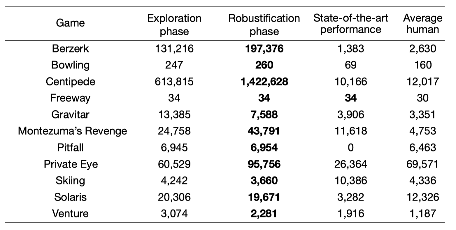
From Figure 2, we can see that, from the selected environments, the robustification phase produces a comparable, sometimes even a better learning algorithm that exceeds the exploration phase.
References
Ecoffet, Adrien, Joost Huizinga, Joel Lehman, Kenneth O Stanley, and Jeff Clune. 2021. “First Return , Then Explore.” Nature 590 (December 2020). https://doi.org/10.1038/s41586-020-03157-9.
Ecoffet, Adrien, Joost Huizinga, Joel Lehman, Kenneth O. Stanley, and Jeff Clune. 2020. “First Return Then Explore.” ArXiv 590 (December 2020). https://arxiv.org/pdf/2004.12919.pdf.