
Introduction
We discuss the For The Win(FTW) agent, proposed by Jaderberg et al. 2019, that achieves human-level performance in a popular 3D team-based first-person video game. The FTW agent utilizes an innovative two-tier optimization process in which a population of independent RL agents is trained concurrently from thousands of parallel matches with agents playing in teams together and against each other on randomly generated environments. In the outer optimization stage, it takes the advantage of the population-based training to evolve internal reward signal, which complements the sparse delayed reward from winning, and hyperparameters, such as the learning rate and weight of individual loss. In the inner loop, it optimizes a temporally hierarchical representation with RNNs operating at different timescales, which enables the agent to reason at multiple timescales.
Task Description
The FTW agent is trained on the Capture The Flag(CTF) environment, where two opposing teams of multiple individual players(they only train with 2 vs 2 games but find the agents generalize to different team sizes) compete to capture each other’s flags by strategically navigating, tagging, and evading opponents. The team with the greatest number of flag captures after five minutes wins.
Environment Observation
The observation consists of \(84\times84\) pixels. Each pixel is represented by a triple of three bytes, which we scale by \({1\over 255}\) to produce an observation \(x\in[0,1]^{84\times84\times3}\). Besides, certain game point signals \(\rho_t\), such as I picked up the flag, are also available.
Action Space
The action space consists of six types of discrete partial actions:
- Change in yaw rotation with five values \(\text{(-60, -10, 0, 10, 60)}\)
- Change in pitch with three values \(\text{(-5, 0, 5)}\)
- Strafing left or right (ternary)
- moving forward or backward (ternary)
- tagging or not (binary)
- jumping or not (binary)
This gives us the total number of \(5\times3\times3\times3\times2\times2=540\) composite actions that an agent can produce.
Notations
Here we list some notations that will be used in the rest of the post for better reference
- \(\phi\): hyperparameters
- \(\pi\): agent policy
- \(\Omega\): CTF map space
- \(r=\pmb w(\rho_t)\): intrinsic reward
- \(p\): player \(p\)
- \(m_p(\pi)\): a stochastic matchmaking scheme that biases co-players to be of similar skill to player \(p\), see Elo scores in Supplementary Materials for details of scoring agent’s performance
- \(\iota\sim m_p(\pi)\): co-players of \(p\)
FTW Agent
Overall
There are three challenges in Capture the Flag:
- CTF play requires memory and long-term temporal reasoning of high-level strategy.
- The reward is sparse—only at the end of the game will the reward be given, therefore the credit assignment problem is hard.
- The environment setups are varied from match to match. Besides different maps, there could be a different number of players, level of teammates, etc.
The FTW agent meets the first requirement by introducing an architecture that features a multi-timescale representation, reminiscent of what has been observed in the primate cerebral cortex, and an external working memory module, broadly inspired by human episodic memory. The credit assignment problem is addressed by enabling agents to evolve an internal reward signal based on the game points signal \(\rho_t\). Finally, to develop diverse generalizable skills that are robust to different environment setups, we concurrently train a large diverse population of agents who learn by playing with each other in different maps. This diverse agent population also paves a way to perform population-based training on the optimization of internal rewards and hyperparameters.
Temporally Hierarchical Reinforcement Learning
Architecture
The FTW agent uses a hierarchical RNN with two LSTMs operating at different timescale(although this architecture can be extended to more layers, Jaderberg et al. 2019 found in practice more than two layers made little difference on the task). The fast ticking LSTM, which evolves at each timestep, outputs the variational posterior \(\mathbb Q(z_t\vert \mathbb P(z_t^p),z_{<t},x_{\le t}, a_{<t}, r_{<t})=\mathcal N(\mu_t^q,\Sigma_t^q)\). \(z_t\) sampled from \(\mathcal N(\mu_t^q,\Sigma_t^q)\) is then used as the latent variable for policy, value function, and auxiliary tasks. The slow timescale LSTM, which updates every \(\tau\) timesteps, outputs the latent prior \(\mathbb P(z_t^p\vert z_{<\tau\lfloor{t\over\tau}\rfloor}^p, x_{\le\tau\lfloor{t\over\tau}\rfloor}, a_{<\tau\lfloor{t\over\tau}\rfloor}, r_{<\tau\lfloor{t\over\tau}\rfloor})=\mathcal N(\mu_t^p,\Sigma_t^p)\). This prior distribution, as we will explain soon, then serves as a regularization to the variational posterior. Intuitively, the slow LSTM generates a prior on \(z\) which predicts the evolution of \(z\) for subsequent \(\tau\) steps, while the fast LSTM generates a variational posterior on \(z\) that incorporates new observations but adheres to the predictions made by the prior. The following figure summarizes this process at timestep \(t\), and we will append a more detailed figure from the paper in Supplementary Materials.
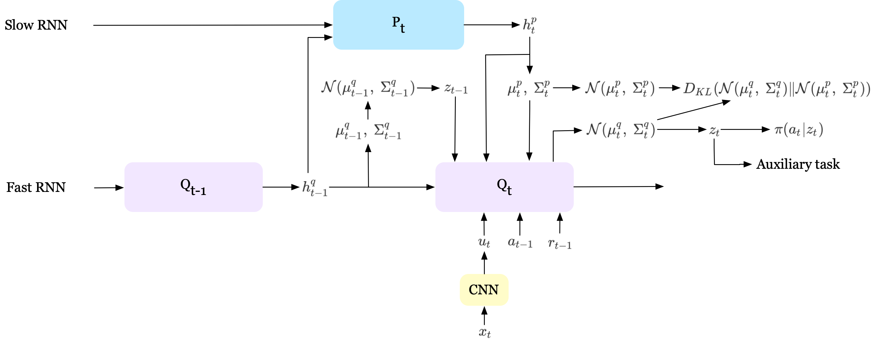
Mathematically, we can express the evolution of the hidden states of both fast and slow RNNs as follows
\[\begin{align} \text{Fast LSTM}&\qquad\qquad h_t^q=g_q(u_t,a_{t-1},r_{t-1},h_t^p,h_{t-1}^q,\mu_t^p,\Sigma_t^p,z_{t-1})\\\ \text{Slow LSTM}&\qquad\qquad h_t^p=\begin{cases}g_p(h_{t-1}^q, h_{t-\tau}^p)&\mathrm{if}\ t\mod\tau=0\\\ h_{\tau\lfloor{t\over\tau}\rfloor}^p&\mathrm{otherwise}\end{cases} \end{align}\]where \(g_p,\ g_q\) are slow and fast timescale LSTM cores, respectively.
Objectives
The FTW uses almost the same loss function as UNREAL with V-trace for off-policy correction and additional KL terms for regularization.
\[\begin{align} \min\mathbb E_{z_t\sim\mathbb Q}&[\mathcal L(z_t,x_t)]+\lambda_{KL}D_{KL}(\mathcal N(\mu_{t}^q,\ \Sigma_{t}^q)\Vert \mathcal N(\mu_{t}^p,\ \Sigma_{t}^p))+\lambda_{KL2}D_{KL}(\mathcal N(\mu_t^p,\Sigma_t^p\Vert\mathcal N(0, 0.1^2)))\tag {1}\\\ where\quad \mathcal L(z_t,x_t)&=\mathcal L_{IMPALA}+\underbrace{\lambda_{PC}\sum_c\mathcal L_{PC}+\lambda_{RP}\mathcal L_{RP}}_\text{auxiliary objectives from UNREAL}\\\ \quad \mathcal L_{IMPALA}&=\mathcal L_\pi+0.5\mathcal L_V-\lambda_{\mathcal H}\mathcal H(\pi)\\\ \mathcal L_\pi&=-\rho_t(r_t+\gamma v(x_{t+1},z_{t+1})-V(x_t,z_{t}))\log\pi(a_t|x_t,z_t)\\\ \mathcal L_V&=\big(v(x_{t},z_{t})-V(x_{t},z_{t})\big)^2\\\ v(s_t) &= V(s_t)+\sum_{k=t}^{t+n-1}\gamma^{k-t}\left(\prod_{i=t}^{k-1}c_i\right)\delta_kV\\\ \delta_kV&=\rho_k(r_k+\gamma V(s_{k+1})-V(s_k))\\\ c_{i}&=\min\left(\bar c, {\pi(a_i|s_i)\over \mu(a_i|s_i)}\right)\\\ \rho_k&=\min\left(\bar\rho, {\pi(a_k|s_k)\over \mu(a_k|s_k)}\right)\\\ \mathcal L_{PC}&=\big(r_{t}+\gamma\max_{a'} Q_{PC}(x_{t+1},z_{t+1},a')-Q_{PC}(x_{t},z_{t},a_t)\big)^2\\\ \mathcal L_{RP}&=y_\tau\log f_{RP}(s_{\tau}) \end{align}\]Most parts of the loss have previously been covered back when we discussed UNREAL and IMPALA. The first newly introduced KL term regularizes the posterior latent distribution \(\mathbb Q\) against a prior \(\mathbb P\) following the idea of RL as probabilistic inference. Unlike traditional probabilistic RL methods that directly regularize the policy, Eq.\((1)\) introduces an intermediate latent variable \(z\), which models the dependence on past observations. By regularizing the latent variable, the policy and the prior now differ only in the way this dependence on past observations is modeled. The second KL penalty regularizes the prior policy \(\mathbb P\) against a multivariate Gaussian with mean \(0\) and standard deviation \(0.1\)(see Training Details).
One subtle difference from the previous methods lies in the pixel control policy, denoted as \(\mathcal L_{PC}\) in Eq.\((1)\). In light of the composite nature of the action space, the authors propose training independent pixel control policies for each of the six action groups(see Figure S10(i) in Supplementary Materials for details).
All the coefficients \(\lambda\)s used in Eq.\((1)\) are first sampled from a log-uniform distribution and then are optimized by population-based training.
Intrinsic Reward
The extrinsic reward is only given at the end of a game to indicate winning(+1), losing(-1), or tie(0). This delayed reward poses a prohibitively hard credit assignment problem to learning. To ease this problem, a dense intrinsic reward is defined based on the game point signal \(\rho_t\). Specifically, for each game point signal, agents’ intrinsic reward mapping \(\pmb w (\rho_t)\) is initially sampled independently from \(\mathrm{Uniform}(-1, 1)\). Then these internal rewards are evolved throughout population-based training(PBT), as well as other hyperparameters such as \(\lambda\)s in Eq.\((1)\) and learning rates.
Population-Based Training
Population-based training(PBT) is an evolutionary method that trains a population of models in parallel and constantly replaces the worse models with better models plus minor modifications. In the case of our FTW agent, PBT can be summarized by repeating the following steps
- Step: Each model in the population of \(P=30\) is trained with its hyperparameters for some steps(\(1K\) games). For each game, we first randomly sample an agent \(\pi_p\), and then we select its teammate and opponents based on their Elo scores—see here for a brief introduction to the Elo scores.
- Eval: After the step requirement is met, we evaluate the performance of each model. In the case of FTW, we have the ready agent compete with another randomly sampled agent, and estimate the Elo scores.
- Exploit: If the estimated win probability of the agent was found to be less than \(70\%\), then the losing agent copied the policy, the internal reward transformation, and the hyperparameters of the better agent.
- Explore: We perturb the inherited internal reward and hyperparameters by \(\pm20\%\) with a probability of \(5\%\), except for the slow LSTM time scale \(\tau\), which is uniformly sampled from the integer range \([5,20)\).
Training Details
Agents receive observations from the environment \(15\) times per second. For each observation, the agent returns an action, which repeats four times within the environment. Every training game lasts five minutes, or equivalently, for \(4500\) agent steps. Agents were trained for two billion steps, corresponding to approximately \(450\)K games.
Agents’ parameters were updates every time a batch of \(32\) trajectories of length \(100\) had been accumulated from the arenas in which the respective agents were playing. RMSProp is used as the optimizer with epsilon \(10^{-5}\), momentum \(0\), and decay rate \(0.99\). The learning rate was sampled per agent from \(\text{LogUniform}(10^{-5},5\cdot 10^{-3})\) and further tuned during training by PBT, with a population size of \(30\).
The loss coefficients in Equation \((1)\) are initialized per agent from log-uniform distributions as shown below and then evolved during training by PBT
\[\begin{align} \lambda_{\mathcal H}\sim&\text{LogUniform}(5\cdot10^{-4},10^{-2})\\\ \lambda_{RP}\sim&\text{LogUniform}(0.1,1)\\\ \lambda_{PC}\sim&\text{LogUniform}(0.01,0.1)\\\ \lambda_{KL}\sim&\text{LogUniform}(10^{-3},1)\\\ \lambda_{KL2}\sim&\text{LogUniform}(10^{-4},0.1)\\\ \end{align}\]Due to the composite nature of action space, instead of training pixel control policies directly on \(540\) actions, we train independently pixel control policies for each of the six action groups.
The reward prediction loss was trained using a small replay buffer consisting of \(800\) non-zero-reward and \(800\) zero-reward sequences. Sequences consisted of three observations. The batch size for the reward prediction loss was \(32\), comprised of \(16\) non-zero-reward and \(16\) zero-reward sequences.
A scaling factor on the gradients flowing from fast to slow ticking cores was sampled from \(\text{LogUniform}(0.1, 1)\). The initial slower-ticking core time period \(\tau\) was sampled from \(\text{Categorical}([5,6,\dots,20])\). These quantities are further optimized during training by PBT.
Summary
We can summarize the policy training and PBT as a joint optimization of the following objectives
\[\begin{align} J_{inner}(\pi_p|\pmb w_p)&=\mathbb E_{\iota\sim m_p(\pi), \omega\sim\Omega}\mathbb E_{a\sim\pi_\iota}\left[\sum_{t=0}^T\gamma^t\pmb w_p(\rho_{p,t})\right]\qquad\forall\pi_p\in\pi\\\ J_{outer}(w_p,\phi_p|\pi)&=\mathbb E_{\iota\sim m_p(\pi),\omega\sim\Omega}P(\pi_p^{\pmb w,\pmb\phi} {'} s\ team\ wins|\omega,\pi_{\iota}^{\pmb w,\pmb \phi}) \end{align}\]This can be viewed as a two-tier reinforcement learning problem. The inner optimization, solved with the temporally hierarchical RL, maximizes \(J_{inner}\), the agents’ expected discounted internal rewards. The outer optimization of \(J_{outer}\), solved with PBT, can be viewed as a meta-game, in which the meta-reward of winning the match is maximized w.r.t. internal reward transformation \(\pmb w\) and hyperparameters \(\phi\), with the inner optimization providing the meta transition dynamics.
Experimental Results
Ablation
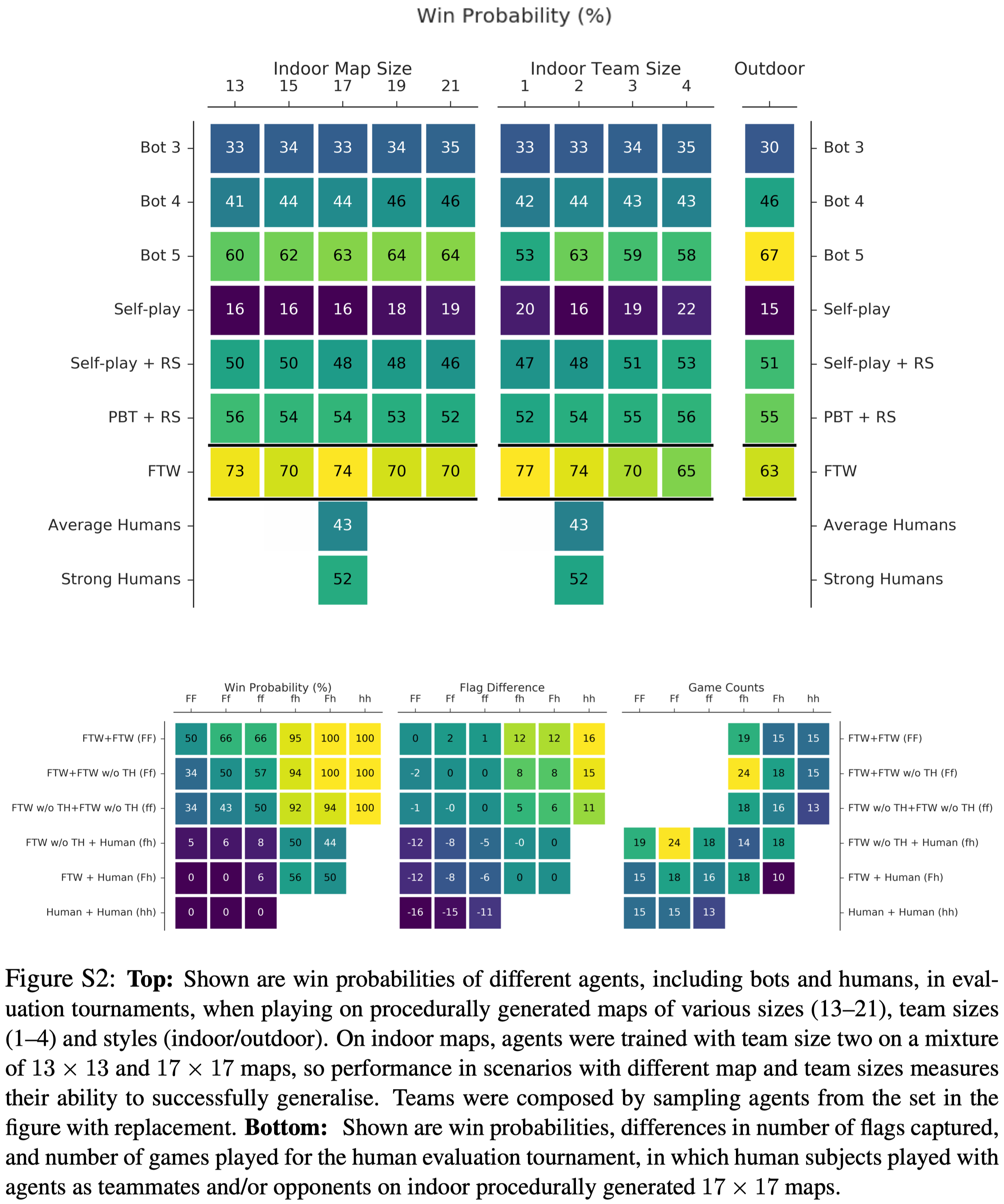
To show the efficacy of each component of FTW agent, we compare the following agents
- Self-play: An agent with an LSTM core trained with loss defined in Equation \((1)\). Four identical agent policies played in each game, two versus two.
- Self-play+reward shaping: Same setup as Self-play above, but with manual reward shaping given by the default system.
- PBT+reward shaping: Same setup as Self-play+reward shaping above, but with a population of agents training against each other in parallel and evolves loss weights during PBT. For each game, the four participating agents were sampled without replacement from the population.
- FTW w/o Temporal Hierarchy: Same setup as PBT+reward shaping above, but with reward shaping replaced by internal reward signals evolved by PBT.
- FTW: The FTW agent, using the recurrent processing core with temporal hierarchy, with matchmaking, PBT, and internal reward signals.
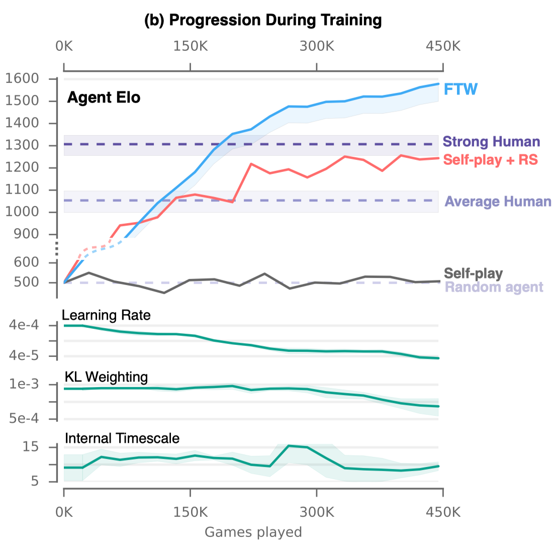
Figure 2 and S2 below show the results of the ablation study.
References
Max Jaderberg, Wojciech M. Czarnecki, Iain Dunning, Luke Marris, Guy Lever, Antonio Garcia Castañeda, Charles Beattie, et al. 2019. “Human-Level Performance in 3D Multiplayer Games with Population-Based Reinforcement Learning.” Science 364 (6443): 859–65. https://doi.org/10.1126/science.aau6249.
Max Jaderberg, Valentin Dalibard, Simon Osindero, Wojciech M Czarnecki, Jeff Donahue, Ali Razavi, Oriol Vinyals, Tim Green, Iain Dunning, Karen Simonyan, et al. Population based training of neural networks. arXiv preprint arXiv:1711.09846, 2017.
Espeholt, Lasse, Hubert Soyer, Remi Munos, Karen Simonyan, Volodymyr Mnih, Tom Ward, Boron Yotam, et al. 2018. “IMPALA: Scalable Distributed Deep-RL with Importance Weighted Actor-Learner Architectures.” In 35th International Conference on Machine Learning, ICML 2018.
Supplementary Materials
Network Architecture

where DNC has been explained in our previous post.
Elo scores
Given a population of \(M\) agents, let trainable variable \(\psi_i\in\mathbb R\) be the rating for agent \(i\). We describe a given match between two players (\(i\), \(j\)) on blue and red, with a vector \(\pmb m\in\mathbb Z^M\), where \(m_i\) is the number of times agent \(i\) appears in the blue team less the number of times the agent appears in the red team—in the Eval step of PBT, where we use two players with \(\pi_i\) on the blue team and two with \(\pi_j\) on the red team, we have \(m_i=2\) and \(m_j=-2\). The standard Elo formula is
\[\begin{align} P(blue\ wins\ against\ red|\pmb m, \psi)={1\over1+10^{-\pmb \psi^T\pmb m/400}} \end{align}\]where we optimize the ratings \(\pmb \psi\) to maximize the likelihood of the data(which we label \(y_i=1\) for ‘blue beats red’, \(y_i={1\over 2}\) for draw, and \(y_i=0\) for ‘red beats blue’). Since win probability is determined only by absolute difference in ratings we typically anchor a particular agent to a rating of \(1000\) for ease of interpretation.
The teammate&oppoents’ sampling distribution for a particular agent is defined as
\[\begin{align} P(\pi|\pi_p)\propto{1\over\sqrt{2\pi\sigma^2}}\exp\left(-{(P(\pi_p\ beats\ \pi|\phi)-0.5)^2\over 2\sigma^2}\right)\qquad where\ \sigma={1\over 6} \end{align}\]which is a normal distribution over Elo-based probabilities of winning, centered on agents of the same skill(\(\mu=0.5\)).