GCL — Guided Cost Learning

Introduction

In reinforcement learning, rewards serve as a guide that indicates the agent what they should do or achieve in a specific environment. In many cases, reward functions are designed by humans to embody the desired behavior that one expects the agent to achieve. However, in many real-world scenarios, such as robotics, dialog, autonomous driving etc., it is generally hard to design an appropriate reward function. Instead, it might be easier to collect some expert data instead. Inverse reinforcement learning aims to utilize expert data so as to infer the reward function. In this post, we will talk about a Maximum Entropy Inverse Reinforcement Learning(MaxEnt IRL) algorithm, namely Guided Cost Learning(GCL), that learns the reward function from expert data.

Preliminaries

Problem Setup

In the setting of IRL, we generally have states space \(\mathcal S\), action space \(\mathcal A\), samples \({\tau_i}\) from some (near-)optimal policy \(\pi^*\), and sometimes dynamics model \(p(s’\vert s,a)\) at our disposal. The goal is to recover the desired reward function and whereby to learn the policy. This is challenging in that it is difficult to evaluate a learned reward, and the expert data in some cases may not be that kind of “expert” (people may be lazy and distracted).

Why Should We Learn The Reward

One might ask: If we have the expert data, why do we bother the reward function? Why don’t we apply imitation learning to directly mimic the expert? This actually works decently well in many cases, but it has some deficiencies:

Aping the expert’s behavior does not necessarily capture the salient parts of the behavior—the agent simply attempts to reproduce the behavior, but does not try to figure out the reasoning or logic behind it. This may not be desirable because some parts may be obviously more important than others.
In some cases, the agent might not have the same capability as the expert. That is, the agent may not even be possible to mimic the expert. If the agent can figure out the goal, then the agent may optimize the goal with its own capability—it might do the task differently, but still achieving the same outcome.
Imitation learning follows maximum likelihood pattern, which could be problematic in many cases. Especially, when the model does not have the capability to represent the entire data distribution, maximizing likelihood exhibits moment-matching behavior, which will lead to a distribution that “covers” all of the modes but puts most of its mass in parts of the space that have negligible density under the data distribution. Instead, it may be preferable in many scenarios to exhibit mode-seeking behavior, by either minimizing the backward KL divergence between two distribution (which we will see later in guided cost learning) or training a generative model adversarially (which will be more clear when we see the connection between MaxEnt IRL and GANs in the next post). A model with mode-seeking behavior tries to “fill in” as many modes as it can, without putting much mass in the space in between.

The Probabilistic Graphical Model of Decision Making

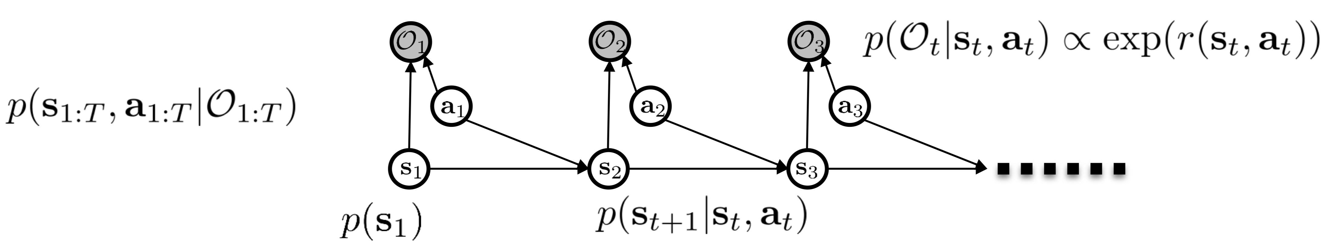
In our previous post, we have discussed a probabilistic graphical model (PGM, as shown above) that allows us to model suboptimal behavior. In this model, we introduce an additional set of Boolean variables called optimality variables \({O_i}\) to indicate whether the given state-action pair is optimal. The probability that the optimality variable is true given a state-action pair is proportional to the exponential of the reward function, i.e., \(p(O_t\vert s_t,a_t)\propto \exp(r(s_t,a_t))\). Our objective before was to answer the question: what the trajectory might be if the agent acts optimally, i.e., \(p(s_{1:T}, a_{1:T}\vert O_{1:T}=1)\).

In this post, we will further explore this model, but now we have the optimal trajectories, and our objective is to figure out what the reward function would be given these optimal trajectories. Or in other words, what is the reward function that maximizes the probability of given trajectories. This is actually the standard problem setup that we can solve using maximum likelihood estimation.

Guided Cost Learning

Recall that the trajectory distribution provided that the agent acts optimally is proportional to the exponential of total rewards:

\[\begin{align} p(\tau|O_{1:T})&\propto p(\tau)\exp(r_\psi(\tau)) \end{align}\]

where \(p(\tau)=p(s_1)\prod_{t=1}^{T-1}p(s_{t+1}\vert s_t,a_t)\), and we here parametrize the reward function by parameter \(\psi\). Noticing that we are computing probabilities here, the above result can be renormalized as follows

\[\begin{align} p(\tau|O_{1:T})={1\over Z}p(\tau)\exp(r_\psi(\tau))\tag {1} \end{align}\]

where the partition function \(Z=\int p(\tau)\exp(r_\psi(\tau))d\tau\).

As a side note, if we merge \(p(\tau)\) into \(Z\), which is fine since we are considering the reward function here, then we will get a Boltzmann distribution,

\[\begin{align} p(\tau|O_{1:T})={1\over Z}\exp(r_\psi(\tau))\tag {2} \end{align}\]

which is commonly used as the objective of MaxEnt IRL in literature. In this post, however, we stick with Eq.\((1)\) since it will give us a better sense of what is going on here. But all the following discussions should work with Eq.\((2)\) with a little adjustment.

MaxEnt IRL is essentially an maximum likelihood estimation(MLE) problem, in which we maximize the log-likelihood of the demonstration probability (Eq.\((1)\)) w.r.t. the parameters \(\psi\) in the reward function:

\[\begin{align} \max_\psi\mathcal L_r(\psi)&=\max_\psi{1\over N}\sum_i\log p(\tau_i|O_{1:T})\\\ &=\max_\psi{1\over N}\sum_{i=1}^Nr_\psi(\tau_i)+\log p(\tau_i)-\log Z\\\ &=\max_\psi{1\over N}\sum_{i=1}^Nr_\psi(\tau_i)-\log Z\tag {3} \end{align}\]

It is easy to compute the first term, the total rewards of expert trajectories, but the second term is troublesome. To get a better sense of what it represents, let us take the gradient of Eq.\((3)\) w.r.t. \(\psi\):

\[\begin{align} \nabla_\psi \mathcal L&={1\over N}\sum_{i=1}^N\nabla_\psi r(\tau_i)-\int {1\over Z}p(\tau)\exp(r_\psi(\tau))\nabla_\psi r_\psi(\tau)d\tau\\\ &=\mathbb E_{\tau\sim\pi^\*(\tau))}[\nabla_\psi r_\psi(\tau)]-\mathbb E_{\tau\sim p(\tau|O_{1:T},\psi)}[\nabla_\psi r_\psi(\tau)]\tag {4} \end{align}\]

Eq.\((4)\) provides a nice intuition for the objective defined in Eq.\((3)\): when we maximize the objective, we are encouraging the rewards under the expert policy, and meanwhile penalizing the rewards under the soft optimal policy for the current reward function. The latter makes sense since the soft optimal policy for the current reward function is not truly optimal as long as it does not match the expert policy. This gradient also paves the way to approximate the objective Eq.\((3)\): we do so by sampling trajectory rewards from both the expert policy and the soft optimal policy for the current reward function, and then taking the difference between them.

Eq.\((4)\) could work, but it is extremely computationally expensive since we have to compute the soft optimal policy every time the reward is modified. To mitigate this issue, we can instead estimate \(Z\) using a sampling distribution \(q_\theta\) whose policy distribution is \(\pi_\theta\), and correct the bias via importance sampling(as we will see soon, applying importance sampling to \(Z\) gives us a weighted importance sampling version of Eq.\((4)\)). Specifically, we have

\[\begin{align} Z&=\int{p(\tau)\exp(r_\psi(\tau))}d\tau\\\ &=\int p(\tau)\exp(r_\psi(\tau)){q_\theta(\tau,\psi)\over q_\theta(\tau,\psi)}d\tau\\\ &=\mathbb E_{q_\theta}\left[{p(\tau)\exp(r_\psi(\tau))\over q_\theta(\tau,\psi)}\right]\\\ &=\mathbb E_{q_\theta}\left[{p(s_1)\prod_{t=1}^Tp(s_{t+1}|s_t,a_t)\exp(r_\psi(s_t,a_t))\over p(s_1)\prod_{t=1}^Tp(s_{t+1}|s_t,a_t)\pi_\theta(s_t,\psi)}\right]\\\ &\approx{1\over M}\sum_{j=1}^M {\exp(r_\psi(\tau_j))\over \pi_\theta(\tau_j,\psi)}\tag {5} \end{align}\]

where we define the behavior trajectory distribution to be \(q_\theta(\tau,\psi)=p(s_1)\prod_{t=1}^Tp(s_{t+1}\vert s_t,a_t)\pi_\theta(s_t,\psi)\), and \(\tau_j\) is sampled by running policy \(\pi_\theta\). Plugging Eq.\((5)\) back into Eq.\((3)\), and taking gradient, we will have the weighted importance sampling version of Eq.\((4)\), which reduces the variance of the gradient while introducing a little bit of bias (Section 5.5 of Sutton & Barto Book).

\[\begin{align} \nabla_\psi\mathcal L&\approx{1\over N}\sum_{i=1}^N\nabla_\psi r(\tau_i)-{1\over Z_w}\sum_{j=1}^Mw_j\nabla_\psi r_\psi(\tau_j)\tag {6}\\\ \mathrm{where}\quad w_j&={\exp(r_\psi(\tau_j))\over \pi_\theta(\tau_j,\psi)}\\\ Z_w&=\sum_{j=1}^Mw_j \end{align}\]

Eq.\((6)\) frees us from the need of a soft optimal policy for the current reward, but it introduces another question: what makes a good sampling distribution \(\pi_\theta\)? The statistical answer to the optimal sampling distribution \(q(x)\) for \(E_{p(x)}[f(x)]\) is \(q(x)\propto\vert f(x)\vert p(x)\), in which the variance is at its minimum. The underlying intuition is that we should sample more from where \(\vert f(x)\vert p(x)\) is big and less from where \(\vert f(x)\vert p(x)\) is small. In our case, this suggests that \(\pi_\theta\) should be proportional to \(p(\tau)\exp(r_\psi(\tau_j))\), which is exactly the target objective of the soft optimal policy. Therefore, we minimize the KL divergence between \(\pi_\theta\) and \({1\over Z}\exp(r_\psi(\tau_j))\), obtaining the same objective as the one in MaxEnt RL:

\[\begin{align} \max_\theta \mathcal L_\pi(\theta)=\max_\theta\mathbb E_{\tau\sim \pi_\theta}\left[r_\psi(\tau)+\mathcal H(\pi_\theta(\tau, \psi))\right]\tag {7} \end{align}\]

In practice, the importance sampling estimate defined in Eq.\((5)\) will have very high variance if the sampling distribution \(\pi_\theta\) fails to cover some trajectory \(\tau\) with high values of \(r_\psi(\tau)\), which may result in a large value of the negative-log term in Eq.\((3)\). As a result, the objective will mainly focus on improving the first term and neglect the impact of the second. Because the demonstrations will in general have high reward(as a result of the IRL objective), we can address this coverage problem by mixing the expert demonstrations with the policy samples. Hence, we have the objective

\[\begin{align} \max_\psi\mathcal L_r(\psi)&=\max_\psi{1\over N}\sum_{i=1}^Nr_\psi(\tau_i)-\log Z\tag {8}\\\ \mathrm{where}\quad Z&=\mathbb E_{\tau\sim{1\over 2}\pi^\*+{1\over 2}\pi_\theta}\left[{\exp(r_\psi(\tau))\over {1\over 2}\pi^\*(\tau,\psi)+{1\over 2}\pi_\theta(\tau,\psi)}\right]\\\ &\approx{1\over M}\sum_{j=1}^M{\exp(r_\psi(\tau_j))\over {1\over 2}\pi^\*(\tau_j,\psi)+{1\over 2}\pi_\theta(\tau_j, \psi)} \end{align}\]

where \(\pi(\tau)=\prod_{t=1}^T\pi(a_t\vert s_t)\) and \(r(\tau)=\sum_{t=1}^Tr(s_t,a_t)\). In practice, the demonstration \(\pi^*\) is approximated by a Gaussian trajectory distribution whose parameters are computed from the demonstrations.

Algorithm

Now we formulate the algorithm, which interleaves IRL optimization (Eq.\((8)\)) with a policy optimization procedure (Eq.\((7)\)).

\[\begin{align} &\mathbf{Guided\ Cost\ Learning:}\\\ &\quad \mathrm{Initialize\ policy\ }\pi\\\ &\quad \mathbf{For}\ i=1\mathrm{\ to\ }N:\\\ &\quad\quad \mathrm{Generate\ samples\ }\mathcal D_{samp}\ \mathrm{from\ }\pi\\\ &\quad\quad \mathrm{Sample\ expert\ demonstration}\ \mathcal D_{demo}\\\ &\quad\quad \mathrm{Update\ reward\ function}\ r_\psi\mathrm{\ using\ }\mathcal D_{samp}\mathrm{\ and\ }\mathcal D_{demo}\\\ &\quad\quad \mathrm{Update\ policy\ \pi_\theta\ w.r.t.\ learned\ reward\ function} \end{align}\]

where the policy adopted by the paper is a time-varying linear-Gaussian policy optimized through iLQR.

At the time when the algorithm converges, we get both the desired reward function and an optimal policy w.r.t. the reward function. In this process, we train the reward function with maximum likelihood, but the policy is trained to be mode-seeking because of the mode-seeking behavior of the reverse KL divergence. As a result, even if the policy trained here has the same capacity as one trained with imitation learning, which strictly follows maximum likelihood pattern, its mode-seeking behavior makes it more preferable in practice as long as the reward function is more flexible than the policy[3].

Regularization

Because the reward function is learned from an underspecified objective, regularization should be applied to prevent overfitting. For high-dimensional nonlinear reward function, \(\ell_1\) and \(\ell_2\) regularizers are often insufficient, since different entries in the parameter vector can have drastically different effects on the cost. Finn et al. 2016 propose two regularization terms:

The first term penalizes the local gradient changes, encouraging the reward of demo and sample trajectories to change locally at a constant rate(lcr) by penalizing the second derivative

\[g_{lcr}(\tau)=\sum_{x_t}[(r_\psi(x_{t+1})-r_\psi(x_t))-(r_\psi(x_t)-r_\psi(x_{t-1}))]^2\]

This term reduces high-frequency variation that is often symptomatic of overfitting, making the cost easier to reoptimize.

The second regularizer is more specific to goal-directed episodic tasks, and it encourages the reward of states of a demonstration trajectory to increase monotonically in time using a squared hinge loss

\[g_{mono}(\tau)=\sum_{x_t\in\tau^\*}[\max(0, r_\psi(x_{t-1})-r_\psi(x_{t})-1)]^2\]

The rational behind this regularizer is that, for tasks that consist of reaching a goal, demonstration typically make monotonic progress toward the goal on some manifold.

Recap

Now let us recap what we have gone through. First, we explained why we should learn the reward function. Then we analyzed the optimal trajectory distribution in the probability graphical model and figured that learning reward function is actually an MLE problem. Next, we located the trouble of solving the MLE problem, the partition function \(Z\). By taking the gradient of the objective, we saw that \(\log Z\) could be approximated using the soft optimal policy for the current reward function. However, it was computationally expensive to compute the soft optimal policy every time we updated the reward function. Therefore we employed importance sampling so that we could instead use samples from a behavior policy and correct the bias later. Then we checked out statistical books and found that a desirable behavior policy happens to be the maximum entropy policy, so we simultaneously trained a maximum entropy policy network. In the end, we suggested mixing the expert data and policy samples to compute \(\log Z\) so as to prevent \(-\log Z\) from being unbound.

What is Left?

In the above discussion, we have two optimization procedures — one for the reward and the other for the policy. These two kind of compete with each other: the reward optimization distinguishes demonstrations from policy samples and makes the reward for the policy smaller, while the policy optimization maximizes the policy reward and makes it harder for the reward optimization to distinguish from demonstrations. This competitive nature makes them resemble generative adversarial networks. In the next post, we will further relate IRL to GANs.

References

CS 294-112 at UC Berkeley. Deep Reinforcement Learning Lecture 16
Finn, Chelsea, Pieter Abbeel, Pabbeel Eecs, and Berkeley Edu. 2016. “Guided Cost Learning : Deep Inverse Optimal Control via Policy Optimization” 48.